USING MATLAB: can you answer and explain please and thank you

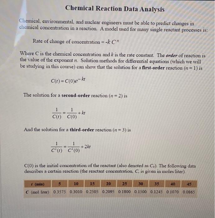
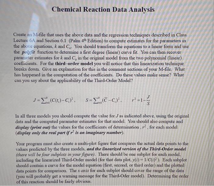
Chemical, environmental, and nuclear engineers must be able to predict changes in chemical concentration in a reaction. A model used for many single reactant processes is: Rate of change of concentration =kCn Where C is the chemical concentration and k is the rate constant. The order of reaction is the value of the exponent n. Solution methods for differential equations (which we will be studying in this course) can show that the solution for a first-order reaction (n=1) is C(t)=C(0)ekt The solution for a second-order reaction (n=2) is C(t)1=C(0)1+kt And the solution for a third-order reaction (n=3) is C2(t)1=C2(0)1+2kt C(0) is the initial concentration of the reactant (also denoted as C0 ). The following data describes a certain reaction (the reactant concentration, C, is given in moles liter). Chemical Reaction Data Analysis Create an M-file that uses the above data and the regression techniques described in Class Lecture 6A and Section 6.1 (Palm 4th Edition) to compute estimates for the parameters in the above equations, k and C0. You should transform the equations to a linear form and use the polyfit function to determine a first degree (linear) curve fit. You can then recover parameter estimates for k and C in the original model from the two polynomial (linear) coefficients. For the third-order model you will notice that this linearization technique breaks down. Give an explanation for this in the comment sections of your M-file. What has happened in the computation of the coefficients. Do these values make sense? What can you say about the applicability of the Third-Order Model? J=i=19(C(ti)Ci)2.S=i=1(CCi)2,r2=1SJ In all three models you should compute the value for J as indicated above, using the original data and the computed parameter estimates for that model. You should also compute and display (print out) the values for the coefficients of determination, r2, for each model (display only the real part if r2 is an imaginary number). Your program must also create a multi-plot figure that compares the actual data points to the values predicted by the three models. and the linearized version of the Third-Order model (there will be four subplots in your figure). There should be one subplot for each model. including the linearized Third-Order model (for that data plot, y(i)=1/C(i)2 ). Each subplot should contain a curve for the model equation (first, second, or third order) and the plotted data points for comparison. The x-axis for each subplot should cover the range of the data (you will probably get a warning message for the Third-Oder model). Determining the order of this reaction should be fairly obvious. Chemical, environmental, and nuclear engineers must be able to predict changes in chemical concentration in a reaction. A model used for many single reactant processes is: Rate of change of concentration =kCn Where C is the chemical concentration and k is the rate constant. The order of reaction is the value of the exponent n. Solution methods for differential equations (which we will be studying in this course) can show that the solution for a first-order reaction (n=1) is C(t)=C(0)ekt The solution for a second-order reaction (n=2) is C(t)1=C(0)1+kt And the solution for a third-order reaction (n=3) is C2(t)1=C2(0)1+2kt C(0) is the initial concentration of the reactant (also denoted as C0 ). The following data describes a certain reaction (the reactant concentration, C, is given in moles liter). Chemical Reaction Data Analysis Create an M-file that uses the above data and the regression techniques described in Class Lecture 6A and Section 6.1 (Palm 4th Edition) to compute estimates for the parameters in the above equations, k and C0. You should transform the equations to a linear form and use the polyfit function to determine a first degree (linear) curve fit. You can then recover parameter estimates for k and C in the original model from the two polynomial (linear) coefficients. For the third-order model you will notice that this linearization technique breaks down. Give an explanation for this in the comment sections of your M-file. What has happened in the computation of the coefficients. Do these values make sense? What can you say about the applicability of the Third-Order Model? J=i=19(C(ti)Ci)2.S=i=1(CCi)2,r2=1SJ In all three models you should compute the value for J as indicated above, using the original data and the computed parameter estimates for that model. You should also compute and display (print out) the values for the coefficients of determination, r2, for each model (display only the real part if r2 is an imaginary number). Your program must also create a multi-plot figure that compares the actual data points to the values predicted by the three models. and the linearized version of the Third-Order model (there will be four subplots in your figure). There should be one subplot for each model. including the linearized Third-Order model (for that data plot, y(i)=1/C(i)2 ). Each subplot should contain a curve for the model equation (first, second, or third order) and the plotted data points for comparison. The x-axis for each subplot should cover the range of the data (you will probably get a warning message for the Third-Oder model). Determining the order of this reaction should be fairly obvious