Using the BMC Model

$1.$ What is Kevin$$s total cost under the optimal plan? How much better is the optimal plan than Kevin$$s

default plan?

$2.$ In the optimal plan, Richmond gets all of its cars from Newark. The per$-$car shipment cost from

Newark to Richmond is $$40,$ and from Jacksonville to Richmond is $$50.$ Suppose the shipment cost

from Newark to Richmond were to increase. How high does the cost have to be for Richmond to start

receiving cars from Jacksonville? $($Hint: Change the cost to $$41$ and re$-$run Solver. If Richmond still

receives all of its cars from Newark, change the cost to $$42$ and re$-$run Solver. Continue until

Richmond receives some cars from Jacksonville.$)$

$3.$ Explain why the shadow price for Newark$$s constraint is $-$$$5.($Hint: What would happen if there were

one more car available at Newark? Re$-$run Solver to find out.$)$ If Kevin could ship one car from

Jacksonville to Newark for $$10,$ would it be worth doing? What if it cost him only $$4?$

$4.$ Explain why the shadow price for Boston$$s constraint is $$35.($Hint: What would happen if demand at

Boston were $101$ rather than $100?$ Re$-$run Solver to find out.$)$ Would Kevin rather see an increase in

demand at Boston or Atlanta?

$5.$ Suppose demand at Richmond were to increase from $80$ to $81$ vehicles. Explain why Kevin$$s total

costs would increase by $$45,$ although it costs $$40$ to send a vehicle from Newark to Richmond, and

$$50$ to send a vehicle from Jacksonville to Richmond. $\backslash$begin$\{$tabular$\}\{|$c$|$c$|$c$|$c$|$c$|$c$|\}$

$\backslash$hline & A & B & C & D & E $\backslash \backslash$

$\backslash$hline $1$ & & INPUTS & & & $\backslash \backslash$

$\backslash$hline $2$ & & City & Supply & Demand & Metric $\backslash \backslash$

$\backslash$hline $3$ & & $(1)$ Newark & $200$ & & units $\backslash \backslash$

$\backslash$hline $4$ & & $(2)$ Boston & & $100$ & units $\backslash \backslash$

$\backslash$hline $5$ & & $(3)$ Columbus & & $60$ & units $\backslash \backslash$

$\backslash$hline $6$ & & $(4)$ Richmond & & $80$ & units $\backslash \backslash$

$\backslash$hline $7$ & & $(5)$ Atlanta & & $170$ & units $\backslash \backslash$

$\backslash$hline $8$ & & $(6)$ Mobile & & $70$ & units $\backslash \backslash$

$\backslash$hline $9$ & & $(7)$ Jacksonville & $300$ & & units $\backslash \backslash$

$\backslash$hline $10$ & & & & & $\backslash \backslash$

$\backslash$hline $11$ & & Per$-$Unit Shipme & Costs & & $\backslash \backslash$

$\backslash$hline $12$ & & Origin & Destination & Cost & $\backslash \backslash$

$\backslash$hline $13$ & & $(1)$ Newark & $(2)$ Boston & $\backslash (\backslash$$ $30\backslash )$ & $\backslash \backslash$

$\backslash$hline $14$ & & $(1)$ Newark & $(4)$ Richmond & $\backslash (\backslash$$ $40\backslash )$ & $\backslash \backslash$

$\backslash$hline $15$ & & $(2)$ Boston & $(3)$ Columbus & $\backslash (\backslash$$ $50\backslash )$ & $\backslash \backslash$

$\backslash$hline $16$ & & $(3)$ Columbus & $(5)$ Atlanta & $\backslash$$$35$ & $\backslash \backslash$

$\backslash$hline $17$ & & $(5)$ Atanta & $(3)$ Columbus & $\backslash (\backslash$$ $40\backslash )$ & $\backslash \backslash$

$\backslash$hline $18$ & & $(5)$ Atlanta & $(4)$ Richmond & $\backslash$$$30$ & $\backslash \backslash$

$\backslash$hline $19$ & & $(5)$ Atlanta & $(6)$ Mobile & $\backslash (\backslash$$ $35\backslash )$ & $\backslash \backslash$

$\backslash$hline $20$ & & $(6)$ Mobile & $(5)$ Atlanta & $\backslash$$$25$ & $\backslash \backslash$

$\backslash$hline $21$ & & $(7)$ Jacksomville & $(4)$ Richmond & $\backslash (\backslash$$ $50\backslash )$ & $\backslash \backslash$

$\backslash$hline $22$ & & $(7)$ Jacksomville & $(5)$ Atlanta & $\backslash (\backslash$$ $45\backslash )$ & $\backslash \backslash$

$\backslash$hline $23$ & & $(7)$ Jacksomville & $(6)$ Mobile & $\backslash (\backslash$$ $50\backslash )$ & $\backslash \backslash$

$\backslash$hline

$\backslash$end$\{$tabular$\}$

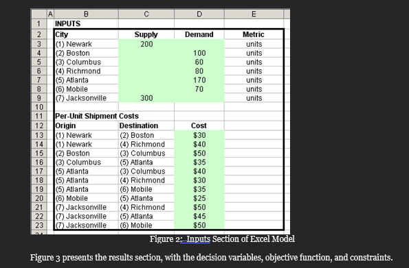
Figure $2$: Inputs Section of Excel Model

Figure $3$ presents the results section, with the decision variables, objective function, and constraints. $\backslash$begin$\{$tabular$\}\{|$c$|$c$|$c$|$c$|$c$|$c$|$c$|\}$

$\backslash$hline & A & B & C & D & E & F $\backslash \backslash$

$\backslash$hline $25$ & & RESULTS & & & & $\backslash \backslash$

$\backslash$hline $26$ & & Decision Variable & Origin & Destination & Amount Shipped & Metric $\backslash \backslash$

$\backslash$hline $27$ & & X$12$ & $(1)$ Newark & $(2)$ Boston & $115$ & units $\backslash \backslash$

$\backslash$hline $28$ & & X$14$ & $(1)$ Newark & $(4)$ Richmond & $85$ & units $\backslash \backslash$

$\backslash$hline $29$ & & $\backslash (\backslash$times $23\backslash )$ & $(2)$ Boston & $(3)$ Columbus & $10$ & units $\backslash \backslash$

$\backslash$hline $30$ & & $\backslash (\backslash$times $35\backslash )$ & $(3)$ Columbus & $(5)$ Atlanta & $2$ & units $\backslash \backslash$

$\backslash$hline $31$ & & X$53$ & $(5)$ Atlanta & $(3)$ Columbus & $55$ & units $\backslash \backslash$

$\backslash$hline $32$ & & $\backslash (\backslash$times $54\backslash )$ & $(5)$ Atlanta & $(4)$ Richmond & $0$ & units $\backslash \backslash$

$\backslash$hline $33$ & & X$56$ & $(5)$ Atlanta & $(6)$ Mobile & $0$ & units $\backslash \backslash$

$\backslash$hline $34$ & & X$65$ & $(6)$ Mobile & $(5)$ Atlanta & $228$ & units $\backslash \backslash$

$\backslash$hline $35$ & & X$74$ & $(7)$ Jacksonville & $(4)$ Richmond & $0$ & units $\backslash \backslash$

$\backslash$hline $36$ & & X$75$ & $(7)$ Jacksonville & $(5)$ Atanta & $0$ & units $\backslash \backslash$

$\backslash$hline $37$ & & X$76$ & $(7)$ Jacksonville & $(6)$ Mobile & $300$ & units $\backslash \backslash$

$\backslash$hline $38$ & & & & & & $\backslash \backslash$

$\backslash$hline $39$ & & Objective Function & & & & $\backslash \backslash$

$\backslash$hline $40$ & & Total Cost & $\backslash (\backslash$$ $30,320\backslash )$ & & & $\backslash \backslash$

$\backslash$hline $41$ & & & & & & $\backslash \backslash$

$\backslash$hline $42$ & & Supply$-$Node Const & traints & & & $\backslash \backslash$

$\backslash$hline $43$ & & City & Outflow$-$Inflow & $\backslash (\backslash$leq $\backslash )$ & Supply & $\backslash \backslash$

$\backslash$hline $44$ & & $(1)$ Newark & $200$ & $\backslash (\backslash$leq $\backslash )$ & $200$ & $\backslash \backslash$

$\backslash$hline $45$ & & $(7)$ Jacksonville & $300$ & $\backslash (\backslash$leq $\backslash )$ & $300$ & $\backslash \backslash$

$\backslash$hline $46$ & & & & & & $\backslash \backslash$

$\backslash$hline $47$ & & Demand$-$Node Cons & straints & & & $\backslash \backslash$

$\backslash$hline $48$ & & City & Inflow$-$Outflow & $\backslash (\backslash$geq $\backslash )$ & Demand & $\backslash \backslash$

$\backslash$hline $49$ & & $(2)$ Boston & $105$ & $\backslash (\backslash$geq $\backslash )$ & $100$ & $\backslash \backslash$

$\backslash$hline $50$ & & $(3)$ Columbus & $63$ & $\backslash (\backslash$geq $\backslash )$ & $60$ & $\backslash \backslash$

$\backslash$hline $51$ & & $(4)$ Richmond & $85$ & $\backslash (\backslash$geq $\backslash )$ & $80$ & $\backslash \backslash$

$\backslash$hline $52$ & & $(5)$ Atlanta & $175$ & $\backslash (\backslash$geq $\backslash )$ & $170$ & $\backslash \backslash$

$\backslash$hline $53$ & & $(6)$ Mobile & $72$ & $\backslash (\backslash$geq $\backslash )$ & $70$ & $\backslash \backslash$

$\backslash$hline

$\backslash$end$\{$tabular$\}$

Figure $3$: Results Section of Excel Model