Using the information provided. Provide me and explain to me how to use a code to plot a strain vs load graph for dynamic loading data.

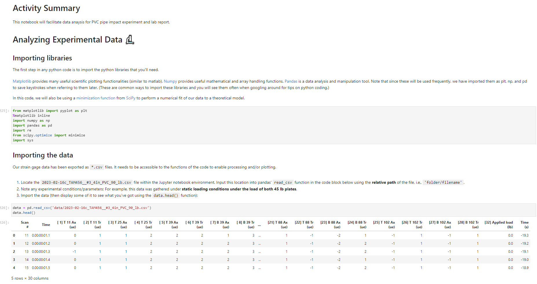
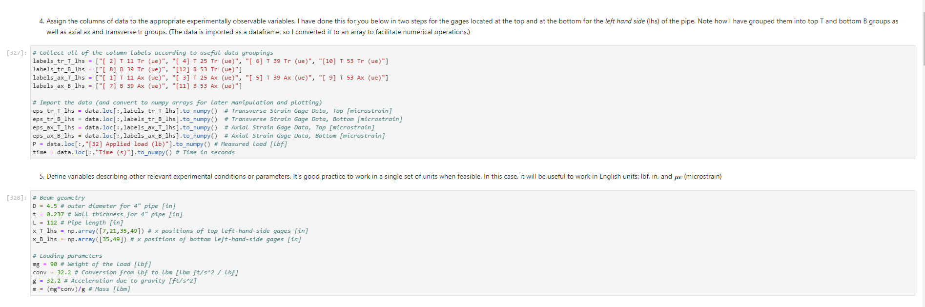
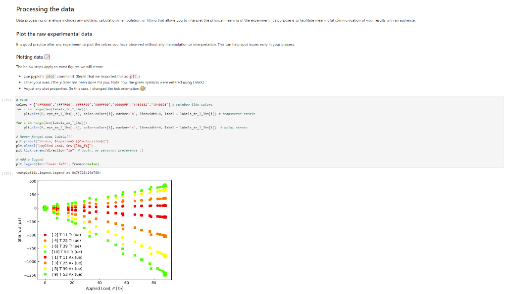
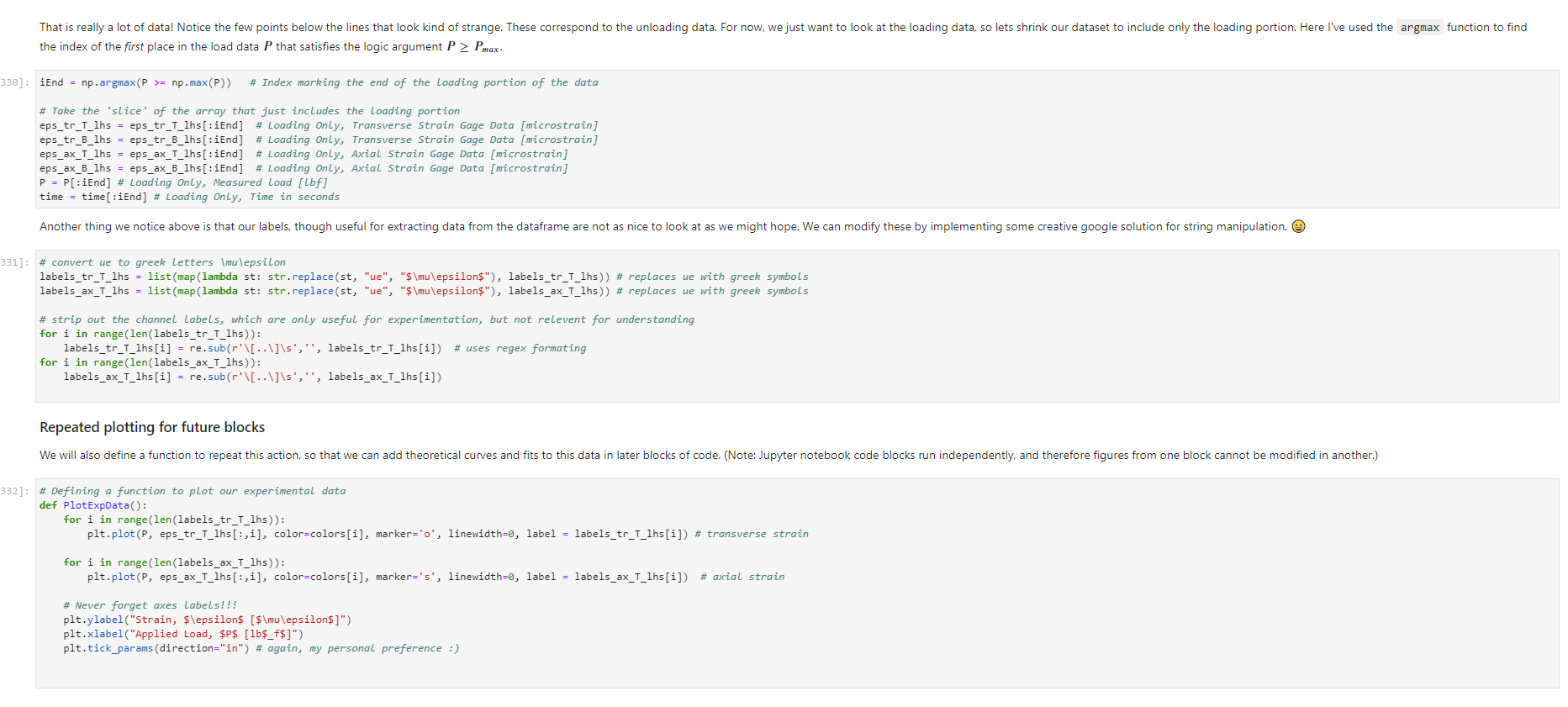
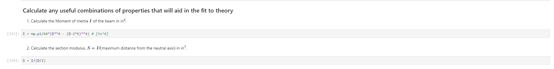
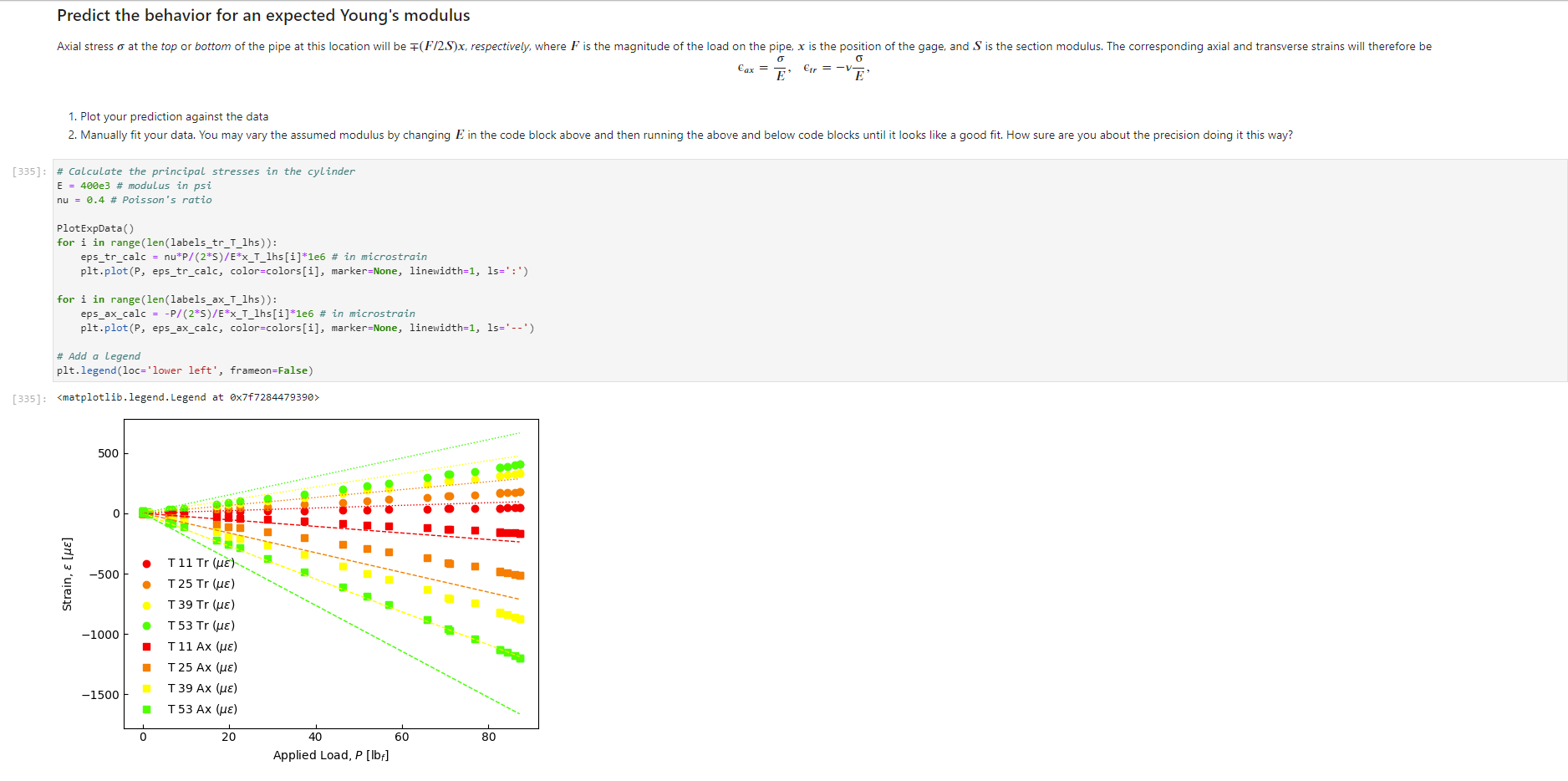
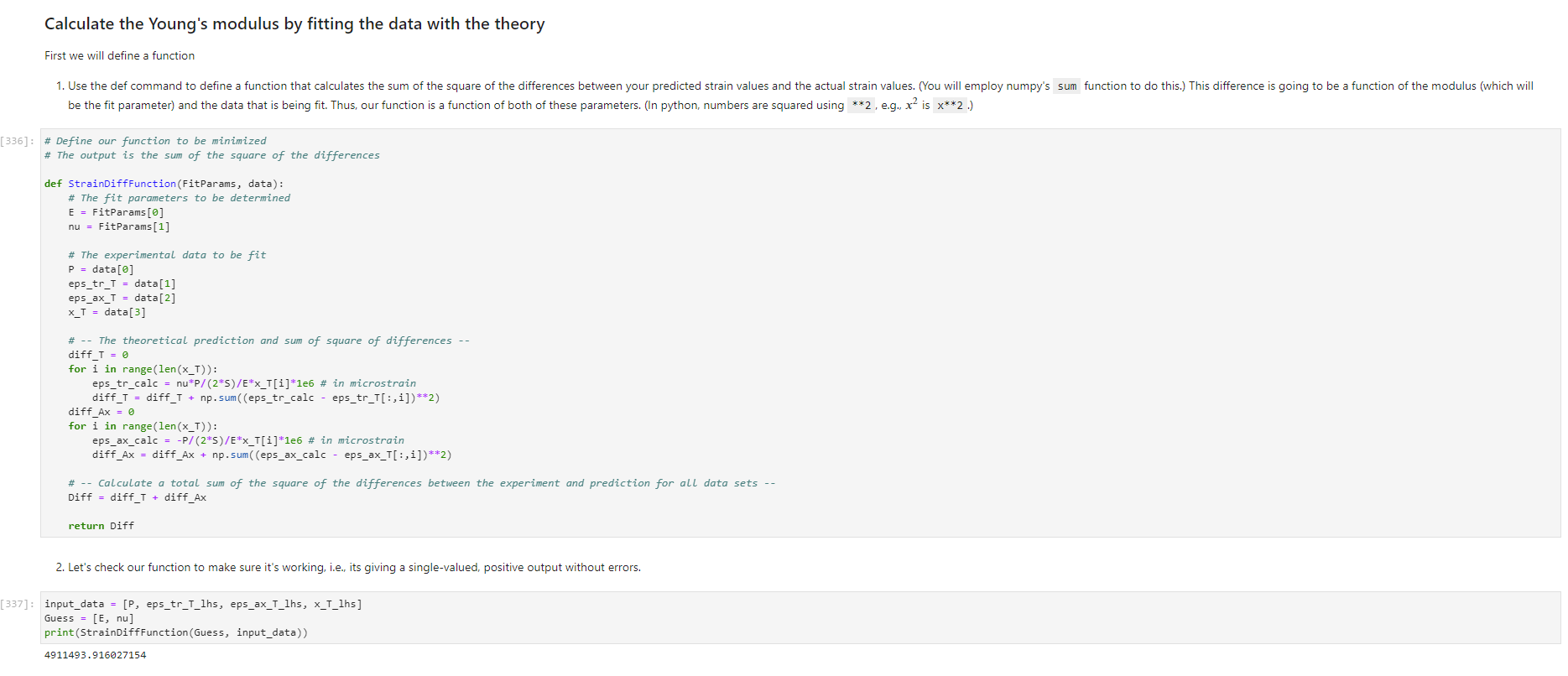
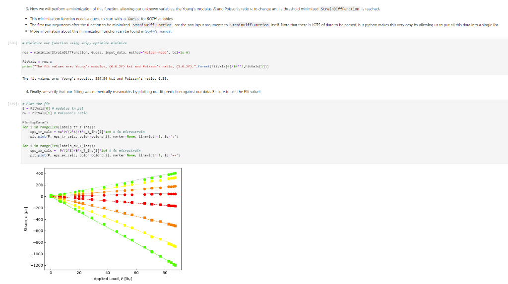
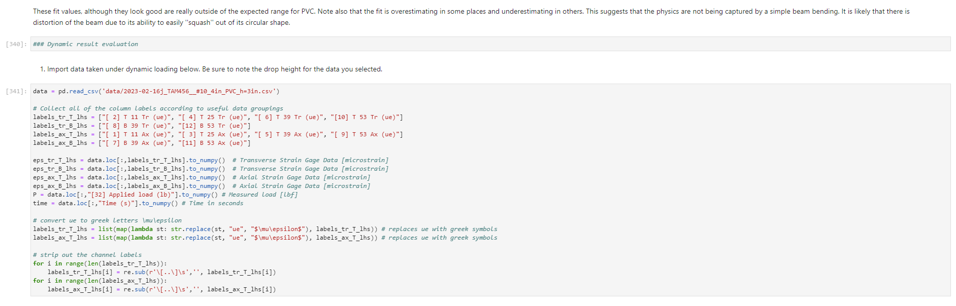
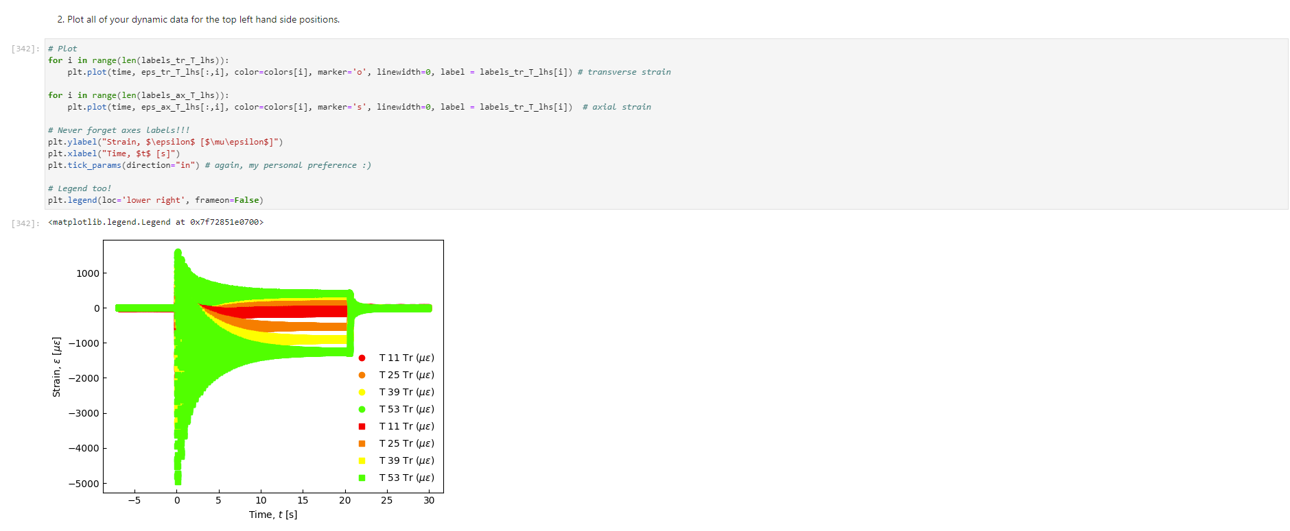
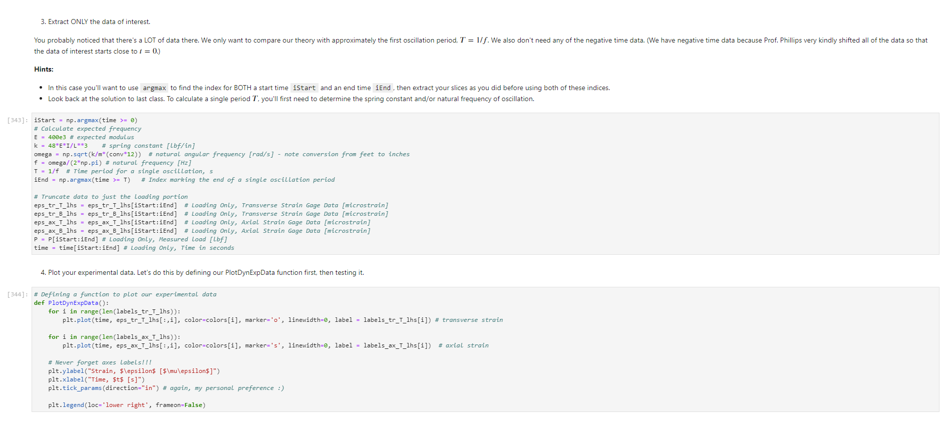
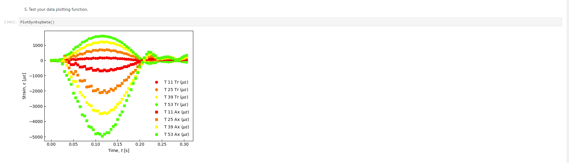
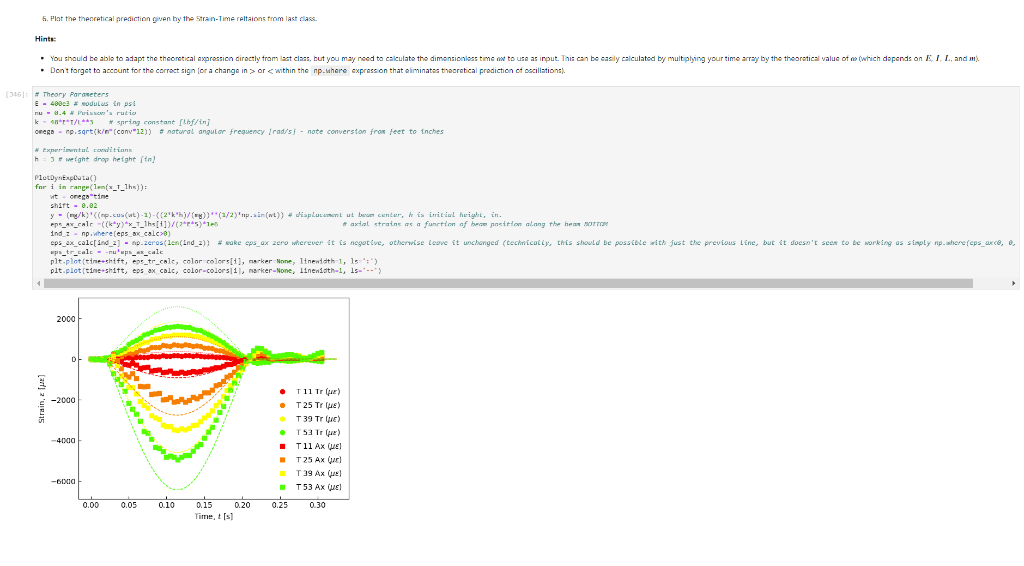
Activity Summary This notebook will facilitate data anaysis for PVC pipe impact experiment and lab report. Analyzing Experimental Data Importing libraries The first step in any python code is to import the python libraries that you'll need. In this code, we will also be using a minimization function from SciPy to perform a numerical fit of our data to a theoretical model. from matplotlib import pyplot as plt \%matplotlib inline import numpy as np import pand import re from scipy.optimize import minimize import sys Importing the data Our strain gage data has been exported as *.csv files. It needs to be accessible to the functions of the code to enable processing and/or plotting. 2. Note any experimental conditions/parameters: For example, this data was gathered under static loading conditions under the load of both 45 lb plates. 3. Import the data (then display some of it to see what you've got using the data.head() function): well as axial ax and transverse tr groups. (The data is imported as a dataframe, so I converted it to an array to facilitate numerical operations.) \# Collect all of the column labels according to useful data groupings labels_tr_T_lhs =["[2]T11Tr (ue)", "[4] T 25Tr (ue)", "[ 6] T 39Tr (ue)", "[10] T 53 Tr (ue)"] labels_tr_B_lhs =["[8] B 39Tr (ue)", "[12] B 53Tr (ue)"] labels_ax_T_lhs =["[1] T 11Ax (ue)", "[ 3 ] T 25Ax (ue)", "[ 5] T 39Ax (ue)", "[ 9] T 53 Ax (ue)"] labels_ax_B_lhs =["[7] B 39Ax (ue)", "[11] B 53Ax (ue)"] \# Import the data (and convert to numpy arrays for later manipulation and plotting) eps_tr_T_lhs = data.loc[:,labels_tr_T_lhs].to_numpy() \# Transverse Strain Gage Data, Top [microstrain] eps_tr_B_lhs = data.loc[:,labels_tr_B_lhs].to_numpy() \# Transverse Strain Gage Data, Bottom [microstrain] eps_ax_T_lhs = data.loc[:,labels_ax_T_lhs].to_numpy() \# Axial Strain Gage Data, Top [microstrain] eps_ax_B_lhs = data.loc[:,labels_ax_B_lhs].to_numpy() \# Axial Strain Gage Data, Bottom [microstrain] P= data.loc [:," [32] Applied load (1b)].to_numpy () \# Measured Load [lbf] time = data. loc[:, "Time (s)"].to_numpy() \# Time in seconds \# Beam geometry D=4.5 \# outer diameter for 4 pipe [in] t=0.237 \# Wall thickness for 4"pipe [in] L=112 \# Pipe length [ in] x_T_lhs =np.array ([7,21,35,49]) \# x positions of top left-hand-side gages [in] x_B_Ihs = np.array ([35,49])#x positions of bottom left-hand-side gages [in] \# Loading parameters mg=90 \# Weight of the load [lbf] conv =32.2 \#Conversion from lbf to lbm[lbmft/s2/lbf] g=32.2 \# Acceleration due to gravity [ft/s2] m=(mgconv)/g# Mass [Lbm] Processing the data Plot the raw experimental data It is poud peactive after ary experiment to plot the values you have vobserved without amy maripulation of interprelation. This tan help spol issues eariy in your prucess. Plotting data The below steps apply to most figures we will create. - Use pypiat's plat command (Hecall that we imported this as plt.) - Label your axe5. (The y label has been done for you. Note how the greek symhols were entered using lateX.] - Adjust any plot properties. (In this case I changed the tick arientation. Oy) \# PLot for i in range(len(1abele_tr_t_ithe ) : \# Never forget oxes labels?t! p1t.ylate1("Struin, Slupsilun\$ [Simutepsilon ] ) plt.xlake 1 ("Applied land, \$p\$ [1ht_f\$]") plt,tick_porans (dipection- 1n)=gotn, wy persanat preference i) a Aeled a Leysud p1t. 1reend (lar "1nwer left", fremecn-Fm1 ker) the index of the first place in the load data P that satisfies the logic argument PPmax. iEnd =npargmax(P>=npmax(P)) \# Index marking the end of the loading portion of the data \# Take the 'slice' of the array that just includes the loading portion eps_tr_T_lhs = eps_tr_T_lhs[:iEnd] \# Loading Only, Transverse Strain Gage Data [microstrain] eps_tr_B_lhs = eps_tr_B_lhs[:iEnd] \# Loading Only, Transverse Strain Gage Data [microstrain] eps_ax_T_lhs = eps_ax___lhs[:iEnd] \# Loading Only, Axial Strain Gage Data [microstrain] eps_ax_B_lhs = eps_ax_B_lhs[:iEnd] \# Loading Only, Axial Strain Gage Data [microstrain] P=P[:iEnd] \# Loading Only, Measured Load [Lbf] time = time[:iEnd ] Loading Only, Time in seconds \# convert ue to greek letters mulepsilon labels_ax_T_lhs = list(map( lambda st: str.replace(st, "ue", "\$\mulepsilon\$"), labels_ax_T_lhs)) \# replaces ue with greek symbols \# strip out the channel labels, which are only useful for experimentation, but not relevent for understanding for i in range(len(labels_tr_T_lhs)): labels_tr_T_lhs[i] =re.sub(r\\[\]\s,", labels_tr_T_lhs[i]) \# uses regex formating for i in range(len(labels_ax___lhs)): labels_ax_T_lhs [i] = re.sub (r\[\]\s,, , labels_ax_T_lhs[i] ) Repeated plotting for future blocks \# Defining a function to plot our experimental data def PlotExpData(): for i in range(len(labels_tr___lhs)): plt.plot (P, eps_tr_T_lhs[:,i], color=colors[i], marker='o', linewidth=0, label = labels_tr_ , lhs [i]) \# transverse strain for i in range(len(labels_ax_T_lhs)): plt.plot(P, eps_ax_T_lhs[:,i], color=colors[i], marker='s', linewidth=0, label = labels_ax_T_lhs[i]) \# axial strain \# Never forget axes labels!!! plt.ylabel("Strain, \$\epsilon\$ [$\mu\epsilon$]) plt.xlabel("Applied Load, \$P\$[1b\$_f\$]") plt.tick_params(direction="in") \# again, my personal preference :) Calculate any useful combinations of properties that will aid in the fit to theory Predict the behavior for an expected Young's modulus ax=E,tr=vE 1. Plot your prediction against the data [335]: \# Calculate the principal stresses in the cylinder E=400e3 \# modulus in psi nu=0.4 \# Poisson's ratio PlotExpData() for i in range (len(labels_tr___lhs)): eps_tr_calc =nuP/(2S)/ExT lhs [i]1e6# in microstrain plt.plot ( P, eps_tr_calc, color=colors[i], marker=None, linewidth=1, 1s=':') for i in range(len(labels_ax_T_lhs)): eps_ax_calc =P/(2a)/Ex_lhs[i]1e6 \# in microstrain plt.plot (P, eps_ax_calc, color=colors[i], marker=None, linewidth=1, 1s=) \# Add a legend plt. legend (loc='lower left', frameon=False) [335]: Iirst we will define a function be the fit parameter) and the data that is being fit. Thus, our function is a function of both of these parameters. (In python, numbers are squared using 2, e.g., x2 is x2.) Define our function to be minimized The output is the sum of the square of the differences StrainDifffunction(FitParams, data): \# The fit parameters to be determined E= FitParams [0] nu= FitParams [1] \# The experimental data to be fit P=data[] eps_tr_T = data [1] eps_ax_T = data [2] x=data[3] \# -- The theoretical prediction and sum of square of differences -- diff_T =0 for i in range (len(xT)) : eps_tr_calc =nuP/(25)/ExT[i]1e6 \# in microstrain diff_T= diff_\( \left.T+n p . \operatorname{sum}((\text { eps_tr_calc_eps_tr_T[ } T, i])^{* *} 2 ight) \) diff_Ax =0 for i in range (len(xT)) : eps_ax_calc =P/(2S)/Ex_T[i]1e6 \# in microstrain diff_Ax = diff_Ax + np.sum( (eps_ax_calc - eps_ax_T[:,i] )2) \#-- Calculate a total sum of the square of the differences between the experiment and prediction for all data sets -- Diff = diff_ + diff_Ax return Diff 2. Let's check our function to make sure it's working, i.e., its giving a single-valued, positive output without errors. input_data =[P, eps_tr_-_lhs, eps_ax_T_lhs, x_lhs] suess =[E,nu] orint(StrainDifffunction(Guess, input_data)) 911493.916027154 - This minimization furction reeds a quess to start with a Guess for BOTH variables. - More irformation about this minimization function can te found in ScyPy's marual. 4. Miminize our functiun using scipy-aptietize. erimieize res = minLnlef(Straindifffunction, Guess, Input_dats, nethod='Me1der-Mead', tol=1e-6) FitVas = resin The tht values are! Young's modulus, 559.54kss and Polsson's rotio, 0.35. 4. Finally, we verify that eur fitting was numerically ressonable, by plotting our fit prediction against cur data. Be sure to use the elit valuel r plot the ftt E - Fitvals[e] \# sedulus in pst ru - ritvals [1] it Poissan's ratio plotixpinata() for 1 in range ( Len ( labels tr_ T Ihs )}1 for 1 in range (len(labels_ax_T_lhs) ): plt,plot (F, eps_ax_cale, color-colors [1], narker-Wone, 1inenddth=1, 1s=".*) distortion of the beam due to its ability to easily "squash" out of its circular shape. \#\# Dynamic result evaluation 1. Import data taken under dynamic loading below. Be sure to note the drop height for the data you selected. data = pd.read_csv('data/2023-02-16j_TAM456_\#10_4in_PVC_h=3in.csv' ) \# Collect all of the column labels according to useful data groupings labels_tr_T_lhs =["[2] T 11Tr (ue)", "[4] T 25Tr (ue)", "[ 6] T 39Tr (ue)", "[10] T 53Tr (ue)"] labels_tr_B_lhs =[ " [8] B 39Tr (ue)", "[12] B 53Tr (ue)" ] labels_ax_T_lhs =["[ 1] T 11 Ax (ue)", "[ 3] T 25 Ax (ue)", "[5] T 39 Ax (ue)", "[ 9] T 53 Ax (ue)"] labels_ax_B_lhs =[ "[ 7] B 39Ax(ue),"[11] B 53 Ax (ue)"] eps_tr_T_lhs = data.loc[:,labels_tr_T_lhs].to_numpy() \# Transverse Strain Gage Data [microstrain] eps_tr_B_lhs = data.loc[:,labels_tr_B_lhs].to_numpy() \# Transverse Strain Gage Data [microstrain] eps_ax_T_lhs = data.loc [:, labels_ax_T_lhs].to_numpy() \# Axial Strain Gage Data [microstrain] eps_ax_B_lhs = data.loc [:, labels_ax_B_lhs].to_numpy() \# Axial Strain Gage Data [microstrain] P= data.loc [:, "[32] Applied load (1b)].to_numpy () \# Measured Load [lbf] time = data.loc [:, "Time (s)"].to_numpy() \# Time in seconds \# convert ue to greek letters mulepsilon labels_tr_T_lhs = list(map(lambda st: str.replace(st, "ue", "\$\mu\epsilon\$"), labels_tr___lhs)) \# replaces ue with greek symbols labels_ax_T_lhs = list(map(lambda st: str.replace(st, "ue", "\$\mu\epsilon\$"), labels_ax_T_lhs)) \# replaces ue with greek symbols \# strip out the channel labels for i in range(len(labels_tr_T_lhs)): labels_tr___lhs [i]=re.sub(r\[\]\s,, , labels_tr___lhs [i] ) for i in range(len(labels_ax___lhs)): labels_ax_T_lhs[i] =re.sub(r\[\]\s,", labels_ax_T_lhs[i] ) 2. Plot all of your dynamic data for the top left hand side positions. [342]: \# Plot for i in range(len(labels_tr_T_lhs)): plt.plot(time, eps_tr_T_Ihs[:,i], color=colors[i], marker='o', linewidth=0, label = labels_tr_T_lhs[i]) \# transverse strain for i in range(len(labels_ax___lihs)): plt.plot(time, eps_ax_T_Ihs [:,i], color=colors[i], marker='s', linewidth=0, label = labels_tr_T_lhs[i]) \# axial strain \# Never forget axes labels!!! plt.xlabel("Time, $t$[s] ") plt.tick_params(direction="in") \#again, my personal preference :) \# Legend too! plt.legend (loc=' lower right', frameon=False) [342]: matplotlib.legend. Legend at 0x7f72851e0700> 3. Extract ONLY the data of interest. the data of interest starts close to t=0.) Hints: - In this case you'll want to use argmax to find the index for BOTH a start time istart and an end time iEnd, then extract your slices as you did before using both of these indices. - Look back at the solution to last class. To calculate a single period T, you'll first need to determine the spring constant and/or natural frequency of oscillation. istart =npargmax( time >=0) \# Calculate expected frequency E=400e3 \# expected modulus k=48EEI/L3# spring constant [Lbf/in] omega =np.sqrt(k/m( conv*12)) \# natural angular frequency [rad/s] - note conversion from feet to inches f= omega/(2*np.pi) \# natural frequency [Hz] T=1/f \# Time period for a single oscillation, s iEnd =np.argmax( time >=T) \# Index marking the end of a single oscillation period \# Truncate data to just the loading portion eps_tr_T_lhs = eps_tr_T_lhs[istart:iEnd] \# Loading Only, Transverse Strain Gage Data [microstrain] eps_tr_B_lhs = eps_tr_B_lhs[istart:iEnd] \# Loading Only, Transverse Strain Gage Data [microstrain] eps_ax_T_lhs = eps_ax_T_lhs[istart:iEnd] \# Loading Only, Axial Strain Gage Data [microstrain] eps_ax_B_lhs = eps_ax_B_lhs[istart:iEnd] \# Loading Only, Axial Strain Gage Data [microstrain] P=P[ iStart:iEnd ] \# Loading Only, Measured Load [lbf] 4. Plot your experimental data. Let's do this by defining our PlotDynExpData function first, then testing it. \# Defining a function to plot our experimental data def PlotDynExpData(): for i in range(len(labels_tr___lhs)): plt.plot(time, eps_tr_T_lhs[:,i], color=colors[i], marker='o', linewidth=0, label = labels_tr_T_lhs[i]) \# transverse strain for i in range(len (labels_ax___lhs)): plt.plot(time, eps_ax_T_lhs[:,i], color=colors[i], marker='s', linewidth=0, label = labels_ax_T_lhs[i]) \# axial strain \# Never forget axes labels!!! plt.xlabel("Time, \$t\$ [s] ") plt.tick_params(direction="in") \#again, my personal preference :) plt.legend (loc='lower right', frameon=False) 3. Extract ONLY the data of interest. the data of interest starts close to t=0.) Hints: - In this case you'll want to use argmax to find the index for BOTH a start time istart and an end time iEnd, then extract your slices as you did before using both of these indices. - Look back at the solution to last class. To calculate a single period T, you'll first need to determine the spring constant and/or natural frequency of oscillation. istart =npargmax( time >=0) \# Calculate expected frequency E=400e3 \# expected modulus k=48EEI/L3# spring constant [Lbf/in] omega =np.sqrt(k/m( conv*12)) \# natural angular frequency [rad/s] - note conversion from feet to inches f= omega/(2*np.pi) \# natural frequency [Hz] T=1/f \# Time period for a single oscillation, s iEnd =np.argmax( time >=T) \# Index marking the end of a single oscillation period \# Truncate data to just the loading portion eps_tr_T_lhs = eps_tr_T_lhs[istart:iEnd] \# Loading Only, Transverse Strain Gage Data [microstrain] eps_tr_B_lhs = eps_tr_B_lhs[istart:iEnd] \# Loading Only, Transverse Strain Gage Data [microstrain] eps_ax_T_lhs = eps_ax_T_lhs[istart:iEnd] \# Loading Only, Axial Strain Gage Data [microstrain] eps_ax_B_lhs = eps_ax_B_lhs[istart:iEnd] \# Loading Only, Axial Strain Gage Data [microstrain] P=P[ iStart:iEnd ] \# Loading Only, Measured Load [lbf] 4. Plot your experimental data. Let's do this by defining our PlotDynExpData function first, then testing it. \# Defining a function to plot our experimental data def PlotDynExpData(): for i in range(len(labels_tr___lhs)): plt.plot(time, eps_tr_T_lhs[:,i], color=colors[i], marker='o', linewidth=0, label = labels_tr_T_lhs[i]) \# transverse strain for i in range(len (labels_ax___lhs)): plt.plot(time, eps_ax_T_lhs[:,i], color=colors[i], marker='s', linewidth=0, label = labels_ax_T_lhs[i]) \# axial strain \# Never forget axes labels!!! plt.xlabel("Time, \$t\$ [s] ") plt.tick_params(direction="in") \#again, my personal preference :) plt.legend (loc='lower right', frameon=False) 6. Plat the thenretical predintion guen by the Stra n-Time reltaione from last rlass. Hints: * Theary Paraveters E=400s \# soducus in pst. 4 experrinentaL conditians. h=3 t weight drop height [tn] P1atDynexpData() fne i in raner(lan(s_T_lhs )} ut - onegotine eps_ax_calc[ ind z]=np-zeros plt.plot(timensift, epe_te_calc, color-colors [t], narker Mone, 1ineaddth-1, 1s " :*) plt,flot[tine-shitt, eps ax calc, color-colorsi1], narker-None, l1nen1dth-1, 1s