Using the template below, create a python program defines the function do_predprey_simulation() which has eight arguments; these are (1) the initial prey population density x, (2) the initial predator population density y, (3) proportionality constant a, (4) proportionality constant b, (5) proportionality constant c, (6) proportionality constant d, (7) the time-step delta t, and (8) the number of time steps to simulate num_steps. Note the return statement shows that the function is returning a tuple comprising the resulting values of x and y. Complete this function definition by using the equation below where if one knows the values of the two populations x and y at any time t one can estimate their values at a time delta t in the future using the previous rate stipulations. By repeating this process, one can march forward in time computing values of x and y at discrete time points separated by delta t from each other. The answers for x and y respectively should be 0.41 and 28.72

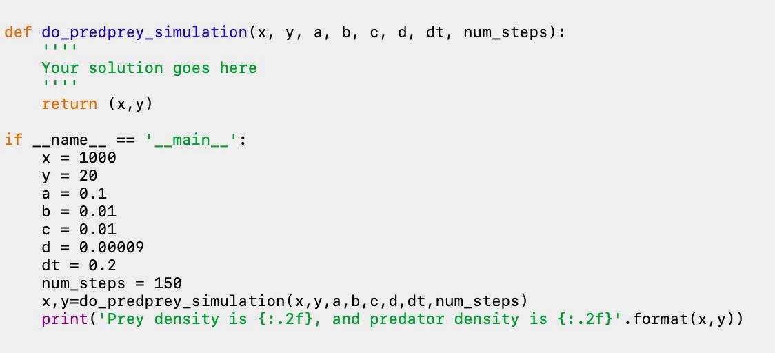
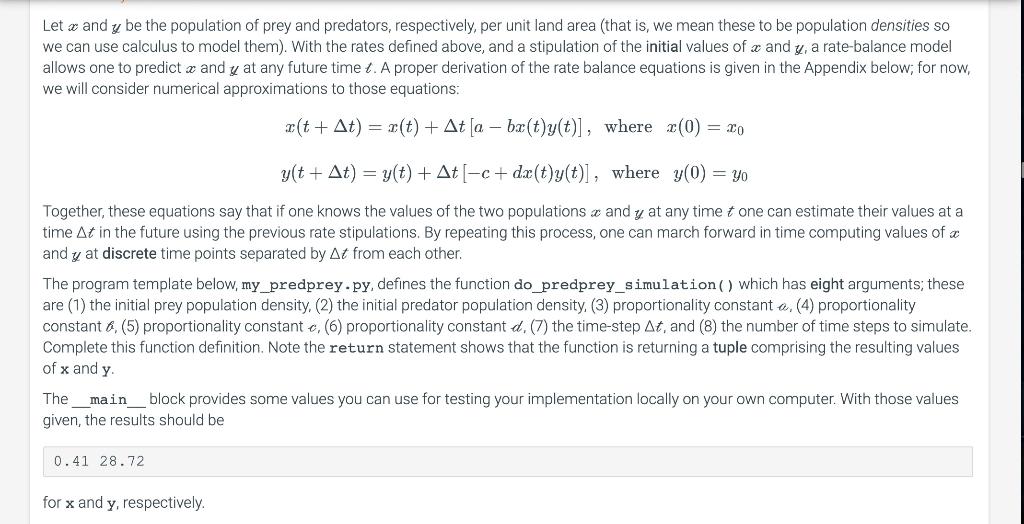
def do_predprey_simulation(x, y, a, b, c, d, dt, num_steps): Your solution goes here return (x,y) if == _name __main__': X = 1000 y = 20 a = 0.1 b = 0.01 C = 0.01 d = 0.00009 dt = 0.2 num_steps = 150 x, y=do_predprey_simulation(x, y, a, b, c, d, dt, num_steps) print("Prey density is {: .2f}, and predator density is {:.2f}'.format(x, y)) Let x and y be the population of prey and predators, respectively, per unit land area (that is, we mean these to be population densities so we can use calculus to model them). With the rates defined above, and a stipulation of the initial values of u and y, a rate balance model allows one to predict x and y at any future time t. A proper derivation of the rate balance equations is given in the Appendix below; for now, we will consider numerical approximations to those equations: 2(t+ At) = 2(t) + At [a b(t)y(t)], where x(0) = 20 y(t + At) = y(t) + At [-c+dx(t)y(t)], where y(0) = yo Together, these equations say that if one knows the values of the two populations x and y at any time t one can estimate their values at a time At in the future using the previous rate stipulations. By repeating this process, one can march forward in time computing values of a and y at discrete time points separated by At from each other. The program template below, my_predprey.py, defines the function do_predprey_simulation) which has eight arguments; these are (1) the initial prey population density, (2) the initial predator population density (3) proportionality constant a, (4) proportionality constant (5) proportionality constant c. (6) proportionality constant d. (7) the time-step At, and (8) the number of time steps to simulate. Complete this function definition. Note the return statement shows that the function is returning a tuple comprising the resulting values of x and y The main block provides some values you can use for testing your implementation locally on your own computer. With those values given, the results should be 0.41 28.72 for x and y, respectively. def do_predprey_simulation(x, y, a, b, c, d, dt, num_steps): Your solution goes here return (x,y) if == _name __main__': X = 1000 y = 20 a = 0.1 b = 0.01 C = 0.01 d = 0.00009 dt = 0.2 num_steps = 150 x, y=do_predprey_simulation(x, y, a, b, c, d, dt, num_steps) print("Prey density is {: .2f}, and predator density is {:.2f}'.format(x, y)) Let x and y be the population of prey and predators, respectively, per unit land area (that is, we mean these to be population densities so we can use calculus to model them). With the rates defined above, and a stipulation of the initial values of u and y, a rate balance model allows one to predict x and y at any future time t. A proper derivation of the rate balance equations is given in the Appendix below; for now, we will consider numerical approximations to those equations: 2(t+ At) = 2(t) + At [a b(t)y(t)], where x(0) = 20 y(t + At) = y(t) + At [-c+dx(t)y(t)], where y(0) = yo Together, these equations say that if one knows the values of the two populations x and y at any time t one can estimate their values at a time At in the future using the previous rate stipulations. By repeating this process, one can march forward in time computing values of a and y at discrete time points separated by At from each other. The program template below, my_predprey.py, defines the function do_predprey_simulation) which has eight arguments; these are (1) the initial prey population density, (2) the initial predator population density (3) proportionality constant a, (4) proportionality constant (5) proportionality constant c. (6) proportionality constant d. (7) the time-step At, and (8) the number of time steps to simulate. Complete this function definition. Note the return statement shows that the function is returning a tuple comprising the resulting values of x and y The main block provides some values you can use for testing your implementation locally on your own computer. With those values given, the results should be 0.41 28.72 for x and y, respectively