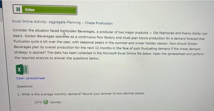
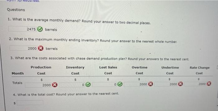
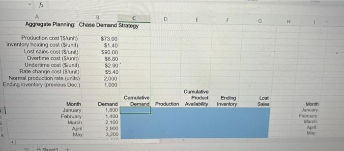
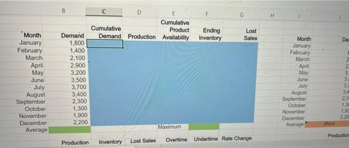
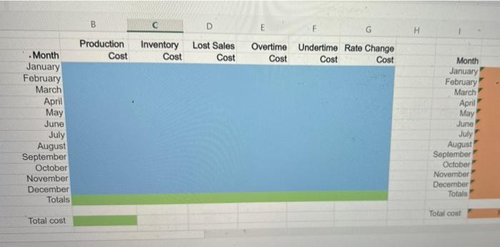
Video Excel Online Activity: Aggregate Planning - Chase Production Consider the situation faced by Golden Beverages, a producer of two major products - Old Fashioned and Foamy Delite root beers, Golden Beverages operates as a continuous flow factory and must plan future production for a demand forecast that fluctuates quite a bit over the year, with seasonal peaks in the summer and winter holiday season. How should Golden Beverages plan its overall production for the next 12 months in the face of such fluctuating demand if the chase demand strategy is applied? The data has been collected in the Microsoft Excel Online file below. Open the spreadsheet and perform the required analysis to answer the questions below. X 11111 Open spreadsheet Questions 1. What is the average monthly demand? Round your answer to two decimal places 2475 barrels Meduleet Questions 1. What is the average monthly demand? Round your answer to two decimal places. 2475 barrels 2. What is the maximum monthly ending Inventory? Round your answer to the nearest whole number. 2000 barrels 3. What are the costs associated with chase demand production plan? Round your answers to the nearest cent. Production Inventory Overtime Rate Change Cost Lost Sales Undertime Month Cost Cost Cost Cost Cost $ Totals $ 2000 5 2000 2000 0 0 2000 4. What is the total cost? Round your answer to the nearest cent. $ fx A Aggregate Planning: Chase Demand Strategy B D E G G H Production cost 7$/unit) Inventory holding cost (S/unit) Lost sales cost (S/unit) Overtime cost (S/unit) Undertime cost (S/unit) Rate change cost (S/unit) Normal production rate (units) Ending inventory (previous Dec.) $73.00 $1.40 $90.00 $6.80 $2.90 $5.40 2.000 1,000 Cumulative Cumulative Product Demand Production Availability Ending Inventory Lost Sales Month January February March April May Demand 1,800 1,400 2,100 2.900 3.200 Month January February March April May 5 7 8 A Shpeti B G H D E Cumulative Cumulative Product Ending Demand Production Availability Inventory Lost Sales De. Month January February March April May June July August September October November December Average Demand 1,800 1,400 2,100 2,900 3,200 3,500 3,700 3,400 2,300 1,300 1,900 2.200 Month January February March April May June July August September October November December Average 3. 30 23 1.30 1.90 2,20 #N/A Maximum Production Production Inventory Lost Sales Overtime Undertime Rate Change B D E H Production Cost Inventory Cost Lost Sales Cost Overtime Undertime Rate Change Cost Cost Cost Month January February March April May June July August September October November December Totals Month January February March April May June July August September October November December Totals Total cost Total cost