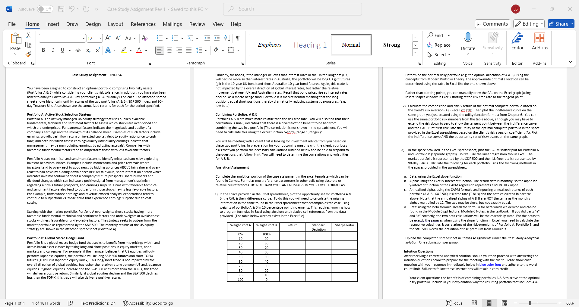
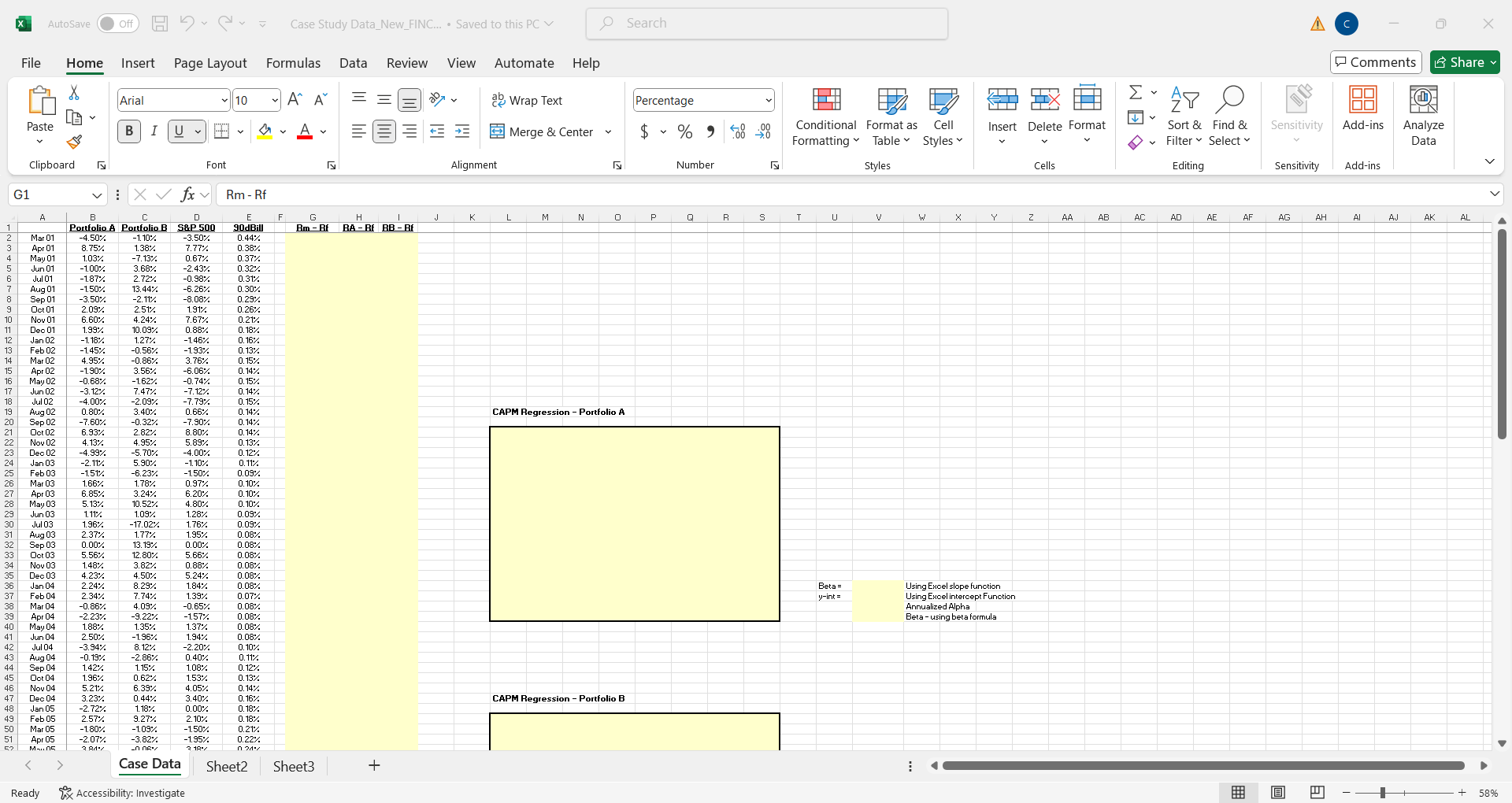
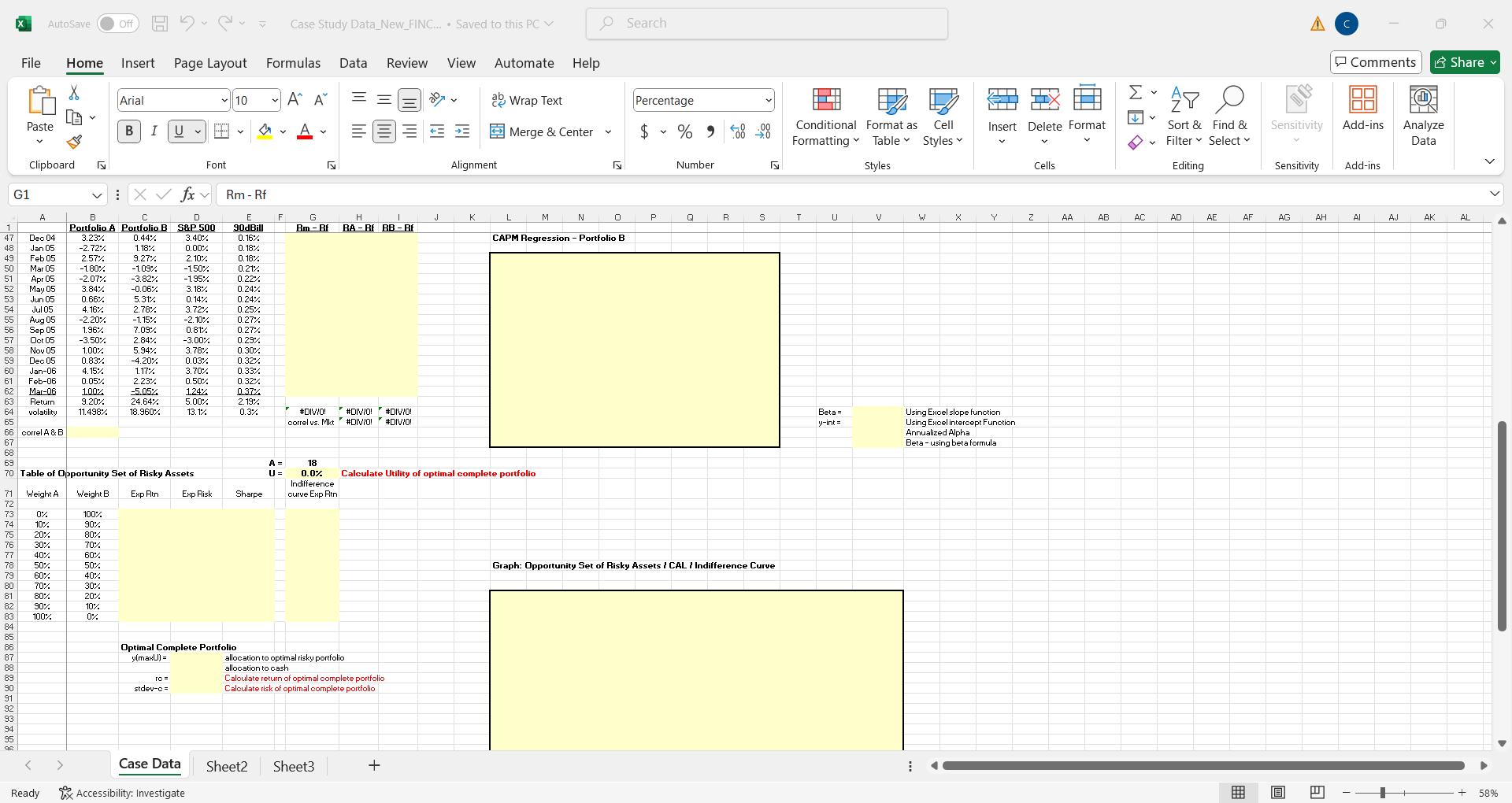
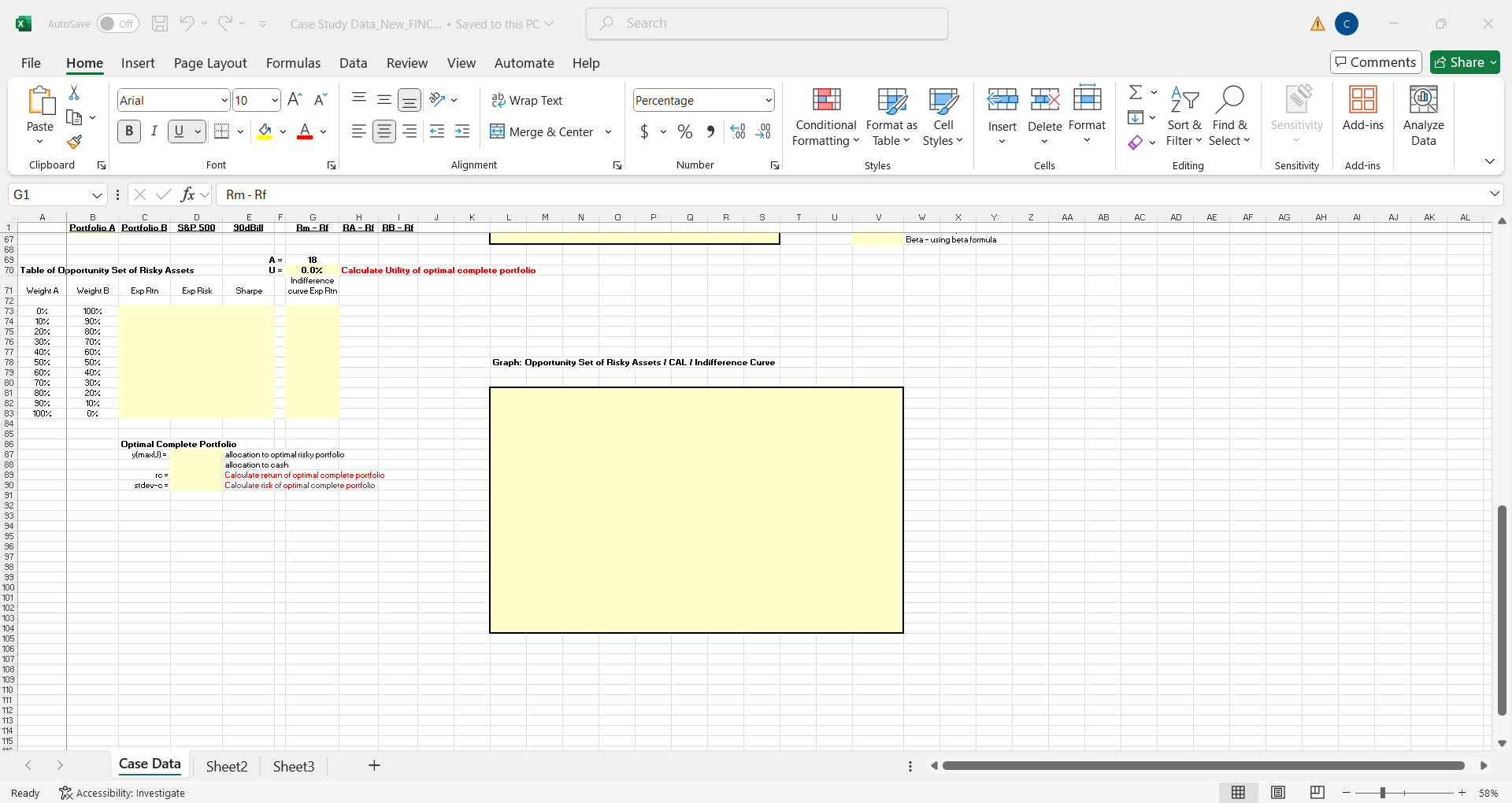
W AutoSave Case Study Assignment Rev 1 . Saved to this PC v Search X File Home Insert Draw Design Layout References Mailings Review View Help Comments Editing Share 12 ~ A" A Aa Ap Find 88 Normal Paste Emphasis c Replace BI Uvab X X A LA Heading 1 Strong Dictate Sensitivity Editor Add-ins Select Clipboard Is Font Paragraph Styles Editing Voice Sensitivity Editor Add-ins Case Study Assignment - FNCE 561 Similarly, for bonds, if the manager believes that interest rates in the United Kingdom (UK) Determine the optimal risky portfolio (e.g. the optimal allocation of A & B) using the will decline more so than interest rates in Australia, the portfolio will be long UK gilt futures concepts from Modern Portfolio Theory. The approximate optimal allocation can be (gilt is the 10-year UK bond) and short Australian 10-year bond futures. Again, this trade is determined using the table in Excel like the one shown above You have been assigned to construct an optimal portfolio comprising two risky assets not impacted by the overall direction of global interest rates, but rather the relative (Portfolios A & B) while considering your client's risk tolerance. In addition, you have also been movement between UK and Australian rates. Recall that bond prices rise as interest rates Rather than plotting points, you can manually draw the CAL on the Excel graph (using asked to analyze Portfolios A & B by performing a CAPM analysis on each. The attached spread decline. As a macro hedge fund, Portfolio B is market neutral meaning that the long Insert Shapes window in Excel) starting at the risk-free rate to the tangent point. sheet shows historical monthly returns of the two portfolios (A & B); S&P 500 Index; and 90- positions equal short positions thereby dramatically reducing systematic exposures. (e.g. day Treasury Bills. Also shown are the annualized returns for each for the period specified. low beta) 2) Calculate the composition and risk & return of the optimal complete portfolio based on the client's risk aversion (A). (Recall ymax!). Then plot the indifference curve on the Portfolio A: Active Stock Selection Strategy Combining Portfolios, A & B same graph you just created using the utility function formula from Chapter 6. You can Portfolio A is an actively managed US equity strategy that uses publicly available Portfolios A & B are much more volatile than the risk-free rate. You will also find that their use the same portfolio risk numbers from the table above, although you may have to undamental, technical and sentiment factors to assess which stocks are over-priced and correlation is small, indicating that there is a diversification benefit to be had from extend the risk down to zero to show the tangent point between the indifference curve which are underpriced. Fundamental factors indicate the magnitude and quality of a combining the two in a portfolio (The correlation is not shown in the spreadsheet. You will and the CAL. Hint: first calculate the utility of the optimal complete portfolio in the space company's earnings and the strength of its balance sheet. Examples of such factors include need to calculate this using the excel function "=corre[(range 1, range2)". provided in the Excel spreadsheet based on the client's risk aversion coefficient (A). Plot earnings growth, cash flow return on invested capital, debt to equity ratio, price to cash the indifference curve AND the opportunity set of risky assets on the same graph. flow, and accruals which assess earnings quality (low quality earnings indicate that You will be meeting with a client that is looking for investment advice from you based on management may be manipulating earnings by adjusting accruals). Companies with these two portfolios. In preparation for your upcoming meeting with the client, your boss favorable fundamental factors tend to outperform those with less favorable factors. asks that you perform the necessary calculations outlined below and be able to respond to In the space provided in the Excel spreadsheet, plot the CAPM scatter plot for Portfolio A the questions that follow. Hint: You will need to determine the correlations and volatilities and Portfolio B (separate graphs). Do NOT use the linear regression tool in Excel. The Portfolio A uses technical and sentiment factors to identify mispriced stocks by exploiting for A & B. market portfolio is represented by the S&P 500 and the risk-free rate is represented by investor behavioral biases. Examples include momentum and price reversals where 90-day T-Bills. Calculate the following for each portfolio using the following methods in investors tend to over-react to good news by bidding up prices ABOVE fair value and over- Analytical Assignment the spaces provided in the spreadsheet: react to bad news by bidding down prices BELOW fair value; short interest on a stock which indicates investor sentiment about a company's future prospects; share buybacks and Complete the analytical portion of the case assignment in the excel template which can be a. Beta: using the Excel slope function dividend changes which can indicate a positive signal from management's optimism found in Canvas. Formulas must reference parameters in other cells using absolute or . Alpha: using the Excel y-intercept function. The return data is monthly, so the alpha via regarding a firm's future prospects; an d earnings surprise. Firms with favorable technical relative cell references. DO NOT HARD CODE ANY NUMBERS IN YOUR EXCEL FORMULAS. y-intercept function of the CAPM regression represents a MONTHLY alpha. and sentiment factors also tend rform those stocks having less favorable factors. Annualized alpha: using the CAPM formula and inputting annualized returns of each For example, firms whose earnings and revenue exceed analysts' expectations tend to 1) In the space provided in the Excel spreadsheet, plot the opportunity set for Portfolios A & portfolio (A & B), S&P 500, risk free rate (T-Bills) and the beta calculated in part "a" continue to outperform vs. those firms that experience earnings surprise due to cost B, the CAL & the indifference curve. To do this you will need to calculate the missing above. Note that the annualized alphas of A & B are NOT the same as the monthly cutting information in the table found in the Excel spreadsheet that accompanies the case using alphas multiplied by 12. The two may be close, but not exactly equal. weights of portfolio A & B in 10 percentage point increments. This requires knowing how d. Beta: using the beta formula. Recall the formula for beta which we derived and can be Starting with the market portfolio, Portfolio A over-weights those stocks having more to program formulas in Excel using absolute and relative cell references from the data found in the Module 6 ppt lecture, Module 6 Notes, & the textbook. If you did parts "a favorable fundamental, technical and sentiment factors and underweights or avoids those provided. (The table below already exists in the Excel file). and "d' correctly, the two beta calculations will be the essentially same. For the betas to stocks with less favorable or un-favorable factors. The strategy seeks to out-perform the be exactly the same as when using the slope function in Excel, you need to calculate the market portfolio as represented by the S&P 500. The monthly returns of the US equity Weight Port A Weight Port B Return Standard Sharpe Ratio respective volatilities & correlations of the risk-premiums of Portfolio A, Portfolio B, and strategy are shown in the attached spreadsheet (Portfolio A). Deviation the S&P 500. Recall the definition of risk-premium from Module 3. 100% Portfolio B: Global Macro Hedge Fund 10 90 Upload the completed spreadsheet in Canvas Assignments under the Case Study Analytical Portfolio B is a global macro hedge fund that seeks to benefit from mis-pricings within and 20 80 Solution. One submission per group across broad asset classes by taking long and short positions in equity markets, bond 70 markets and currencies. For example, if the manager believes that US equities will out- Intuition Questions perform Japanese equities, the portfolio will be long S&P 500 futures and short TOPIX After receiving a corrected analytical solution, should you then proceed with answering the futures (TOPIX is a Japanese equity index). This long/short trade is not impacted by the intuition questions below to prepare for the meeting with the client. Please show each overall direction of global equities, but rather the relative return between US and Japanese question with your response immediately below in blue color font and adhere to the word equities. If global equities increase and the S&P 500 rises more than the TOPIX, this trade count limit. Failure to follow these instructions will result in zero credit. will deliver a positive return. Similarly, if global equities decline and the S&P 500 declines less than the TOPIX, this trade will also deliver a positive return. 1. Your client questions the benefit is of combining portfolios A & B to arrive at the optimal risky portfolio. Include in your explanation why the resulting portfolio that includes A & Page 1 of 4 1 of 1811 words DX Text Predictions: On Accessibility: Good to go " FOCUS 60%W AutoSave Off H Case Study Assignment Rev 1 v Search X File Home Insert Draw Design Layout References Mailings Review View Help Comments Editing Share * 12 ~ A" A Aa Ap Find Times New Roman 88 Emphasis Normal Strong c Replace Paste Heading 1 BI Uvab x x A LA Dictate Sensitivity Editor Add-ins Select Clipboard Font Paragraph Styles Editing Voice Sensitivity Editor Add-ins B has a higher Sharpe Ratio than that of Portfolio (A) or (B) by itself. Prepare a clear & concise response to your client. (Limit response to 75 words) 2. Your client believes in the weak-form of market efficiency as it relates to security selection. Does Portfolio A's performance provide sufficient justification to prove or disprove conclusively your client's belief that markets are weak-form efficient? Why or why not? (Limit response to 100 words) 3. After further discussions with your client, it turns out that she believes markets are semi-strong form efficient as it relates ONLY to stock selection, what portfolio substitution(s) would you make to the recommended optimal risky portfolio and why? No calculations are necessary. (Limit response to 100 words.) 4. After meeting with the client, she informs you that she prefers a return higher than that of the optimal risky portfolio and is willing to accept the higher corresponding risk. a. Is it possible to achieve such a portfolio and if so, how would this be implemented? (Limit response to 50 words) b. What does that indicate about your initial assumption(s) regarding the indifference curve? (Limit response to 50 words) 5. Portfolio A returned 9.20% p.a. over the evaluation period compared to 5.00% p.a. for the S&P 500. This equates to a difference, or outperformance of 4.20% p.a. However, according to CAPM, the annualized alpha of portfolio A is 4.74% p.a. Explain the difference between the two numbers. (Note: It is NOT due to rounding). (Limit responses to 100 words) Upload the completed intuition questions in Canvas under Case Study Intuition Questions. One submission per group. Additional Information The case requires applying investment principals covered throughout the course - specially Modules 4, 5, 6 and calculating geometric returns. It is based on a real-life project an investment management firm did for a large pension client. Each step of the case builds upon the previous, so it is important students get each part of the analysis correct before moving on. If your group is struggling, please let me know ASAP and we can resolve your difficulties preferably via phone. Please do not wait until the last minute to start working on the case. Page 4 of 4 1809 words X Text Predictions: On 2 Accessibility: Good to go " Focus + 60%A X O Search AutoSave Off K vv Case Study Data_New_FINC.. . Saved to this PC v Comments Share File Home Insert Page Layout Formulas Data Review View Automate Help IX Ex AY O ~ 10 ~ A" A " ap Wrap Text Percentage Arial E Sensitivity Add-ins Analyze Conditional Format as Cell Insert Delete Format Sort & Find & $ ~ % " Filter ~ Select Data Paste BI U VFAv Merge & Center Formatting Table Styles ~ Editing Sensitivity Add-ins Styles Cells Font Alignment Number Clipboard G1 viXfx Rm - Rf AA AB AC AD AE AF AG AH Al AJ AK AL K M N P R S U V W X Y 2 B Portfolio A Portfolio B S&P 500 90dBil Bm - Rf BA - Rf BB - Bf Mar 01 4.50% -1. 10% 3.50% 0.44% Apr 01 8.75% 1.38% 7.77% 0.38% lay Of 1.03% -7.13% 0.67% Jun 01 -1.00% 3.68% 2.43% 0.32% 0.31% Jul 07 -1.87%. 2.72%% -0.98% Aug 01 -1.50% 3.44% -6.26% 0.30% jep 01 -3.50% -2.11%% -8.08% 0.292 Oct 01 2.09% 2.51% 1.91% 0.26% Nov 01 6.60% 4.24% 7.67% 0.217 Dec 01 199% 10.09% 1.88% 0. 104 Jan 02 -1.18% 1.27% 1.46% 0.16% Feb 02 -0.56% -1.93%% 0.13% Mar 02 4.95%% -0.86% 3.76%% 0.15% Apr 02 -1.90% 3.56% -6.06%. 0.14% May 02 -0.68% -1.62% -0.74% D.15% Jun 02 -3.12% 7.47% 7.12% 0.14% Jul 02 -4.00% -2.09% -7.79% 0. 15% CAPM Regression - Portfolio A 0.14% Aug U 0.80% 3.40% 0.66% Sep 02 -7.60% 1.32% 7.90% 0.147 Jot 02 6.93% 2.82% 8.80% 0.14% Nov 02 4. 13% 4.95% 5.89% 0.13% Dec 02 -4.99% -5.70% 4.00% . 12% Jan 03 -2. 11% 5.90% -1.10% 0. 11% 25 Feb 03 -1.51% 5.23% -1.50% 0. 09% Mar 03 1.66%% 1.78% 0.97% 0.10% Apr 03 3.85; 3.24% 6.20% 0. 10% May 03 . 137 0.52 4.80% 0. 10% Jun 03 1,11%% 1. 09% 1.28% 0.09% Jul 03 1.96%% -17.02% 1.76% 0.09% Aug 03 37% 1.77 1.95%% 0.08% Sep 03 0.00% 3.19%% 0.00%% 0. 08% Oct 03 5.56% 12.80% 5.667. 1. 08%. 862889 Nov 03 1.48% 3.82% 0.88% 0. 08% 5.24% 0.08% Beta = Using Excel slope function Dec 03 4.23% 4.50% 8.29% 184% D. 08% y-int = Using Excel intercept Function Jan 04 2.24% Annualized Alpha 37 Feb 04 2.34% 7.74%% .39% 0.07% Beta - using beta formula 38 Mar 04 0.86%% 4.09% 0.65% 0. 08% 39 Apr 04 2.23% -9.22%. -1.57% 0.08% May 04 1.88%% 1.35% 1.37% 0. 08% Jun 04 2.50% 1.96%% 1.94%% 0.08% 42 Jul 04 -3.94% 8.12% -2.20%. 0. 107. 43 Aug 04 -0.19% 2.86% 0.40% 0. 11% 44 Sep 04 1.42% 1. 15% 1.08% 0.12% 45 Oct 04 1,96%% 0.62% 1.53% 0.13% 46 Nov 04 5.21% 6.39% 1.05% 0.14% CAPM Regression - Portfolio B 47 Dec 04 3.23% 1.44%% 3.40% 0. 16: 48 Jan 05 2.72% 1.18% 0.00% 0.18: 49 Feb 05 2.57%% 3.27%% 2. 10% 0.18% 50 Mar 05 -1.80% -1.092. 1.50% 0.21% Apr 05 -2.07% -3.827 -1.95% 0.22% MS.. DC Case Data Sheet2 Sheet3 + + 58% Ready Accessibility: InvestigateA AutoSave K vv Case Study Data_New_FINC.. . Saved to this PC v O Search X Off Comments Share File Home Insert Page Layout Formulas Data Review View Automate Help * 10 A" A " E ag Wrap Text Percentage IX Ex AY O Arial Conditional Format as Cell Insert Delete Format Sort & Find & Sensitivity Add-ins Analyze Paste BI U VFAv Merge & Center v $ ~ % " Formatting Table Styles ~ Filter ~ Select Data Styles Cells Editing Sensitivity Add-ins Clipboard Font Alignment Number G1 viX fry Rm - Rf P Q R S U V W X Y 2 AA AB AC AD AE AF AG AH Al AJ AK AL B C M N Portfolio A Portfolio B S&P 500 90dBill Bm - Rf BA - Rf BB - Bf 47 Dec 04 3.23% 0.44% 3.40% 0.16%% CAPM Regression - Portfolio B 48 Jan 05 -2.72% 1.18%% 0.00% 0.18% Feb 05 .57%% 9.27% 2. 10% 0.18% 50 Mar 05 -1.80% -1.09% 1.50% 0.21% 51 Apr 05 -2.07% -3.82% 1.95% 0.227. 52 May 05 3.84% 0.06% 3.18% 0.247 Jun 05 0.66% 5.31 0.14% 0.24% Jul 05 4.16% 2.78% 3.727 0.25% 55 Aug 05 -2.20% -1.15% -2.10% 0.27 Sep 05 1.96% 7.09% 0.81%% 0.27% Oct 05 -3.50% 2.84% -3.00% 0.292 Nov 05 1.00% 5.94%% 3.78% 59 Dec 05 0.83% 4.20% 0.03% 0.32% 60 Jan-06 4. 15% 1.17% 3.70% 0.33%. 61 Feb-06 0.05% 23%% 0.50% 0.32% 62 Mar-Of 100% -5.05% 1.24% 0.37% Return 9.20% 24.64% 5,00% 2.19 Beta = Using Excel slope function 64 volatility 1.498% 18.960% 13. 1% 0.3% #DIV/O! / #DIVIO! / #DIV/O! 65 correl vs. Mkt #DIV/O! " #DIV/O! y-int = Using Excel intercept Function Annualized Alpha 66 correl A & B Beta - using beta formula 67 68 69 18 70 Table of Opportunity Set of Risky Assets 0.0%% Calculate Utility of optimal complete portfolio Indifference Weight A Weight B Exp Rtn Exp Risk Sharpe curve Exp Rtn 72 73 07. 100%% 74 10% 90% 75 20%% 80% 76 30%% 70% 77 60% 78 50% 50% Graph: Opportunity Set of Risky Assets / CAL / Indifference Curve 79 60% 40%% 80 70% 30%% 81 80%% 20%% 82 90% 10%% 83 100% 0%% 85 86 Optimal Complete Portfolio 87 y(maxU) = allocation to optimal risky portfolio 88 allocation to cash 89 Calculate return of optimal complete portfolio 90 stdev-c = Calculate risk of optimal complete portfolio 92 Case Data Sheet2 Sheet3 + + 58% Ready Accessibility: InvestigateAutoSave Off K vv Case Study Data_New_FINC.. . Saved to this PC v O Search A X File Home Insert Page Layout Formulas Data Review View Automate Help Comments Share Arial 10 ~ A" A " E ap Wrap Text Percentage IX Ex AY O Paste BI U VFAv $ ~ % " Conditional Format as Cell Insert Delete Format Sort & Find & Sensitivity Add-ins Analyze Merge & Center Formatting Table Styles v Filter ~ Select Data Clipboard Font Alignment Number Styles Cells Editing Sensitivity Add-ins G1 viXfx Rm - Rf B K M N P R S U V W Y Z AA AB AC AD AE AF AG AH Al AJ AK AL Portfolio A Portfolio B S&P 500 90 dBill Bm - Bf BA - Rf BB - Bf Beta - using beta formula 68 69 A 18 70 Table of Opportunity Set of Risky Assets 0.0% Calculate Utility of optimal complete portfolio Indifference 71 Weight A Weight B Exp Atn Exp Risk Sharpe curve Exp Rtn 72 73 0%% 100% 74 10%% 90% 75 20%% 80% 76 30%% 70% 77 40%% 60% 78 50%% 50% Graph: Opportunity Set of Risky Assets / CAL / Indifference Curve 79 60%% 40% 80 70%% 30%% 80% 20% 82 90%% 10% 83 100% 0 84 86 Optimal Complete Portfolio 87 y(maxU) = allocation to optimal risky portfolio 88 allocation to cash 89 Calculate return of optimal complete portfolio stdev-c = Calculate risk of optimal complete portfolio 91 97 98 99 100 101 102 103 104 105 106 107 108 109 110 115 Case Data Sheet2 Sheet3 + Ready Accessibility: Investigate + 58%