what's wrong here with the calculations? did something go wrong in the capacitor experiment? if so then what do you think happened?Look closely at the (1/C) and time constant data. here's the procedure :

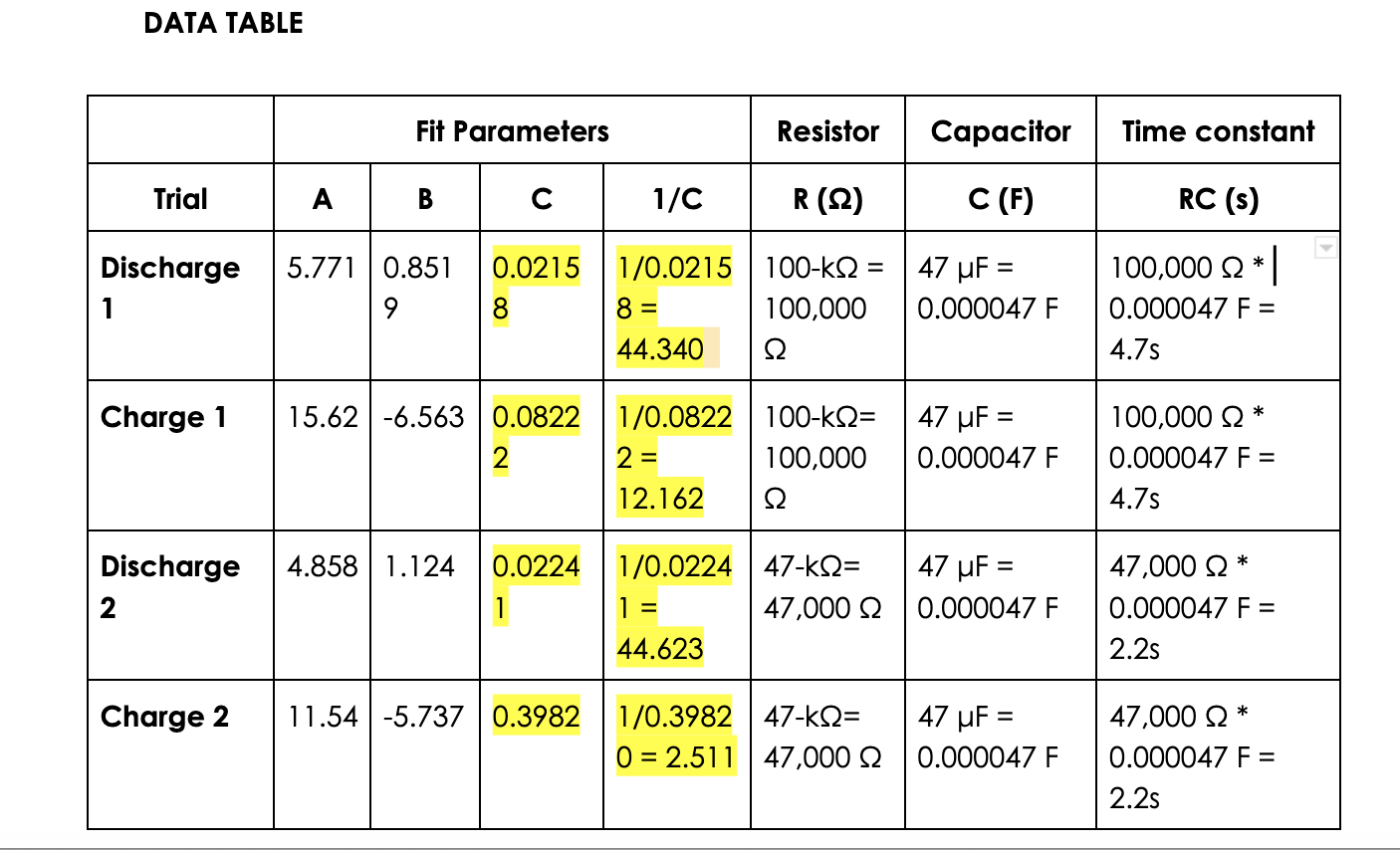
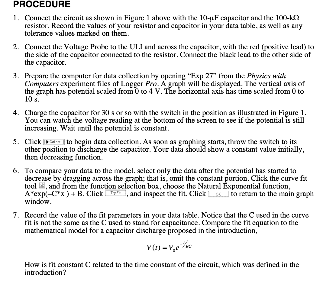
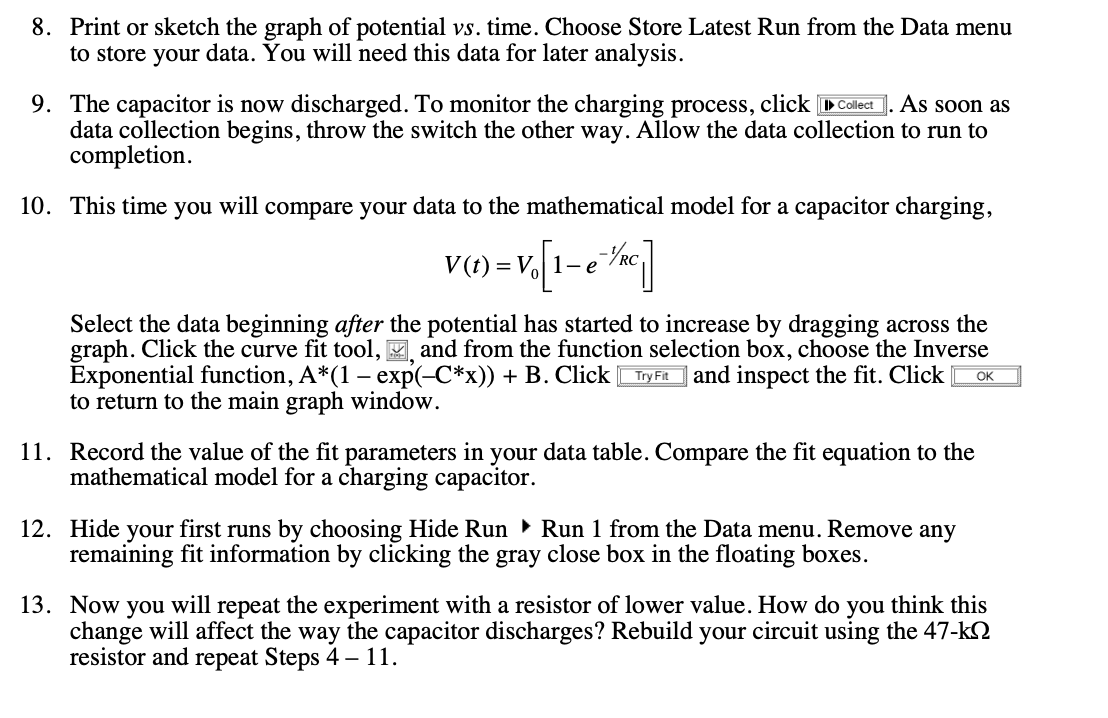
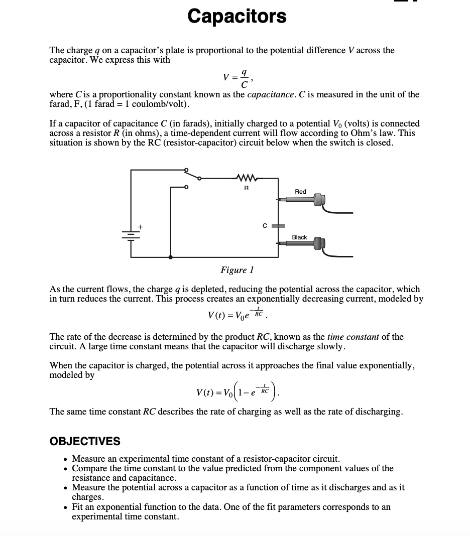
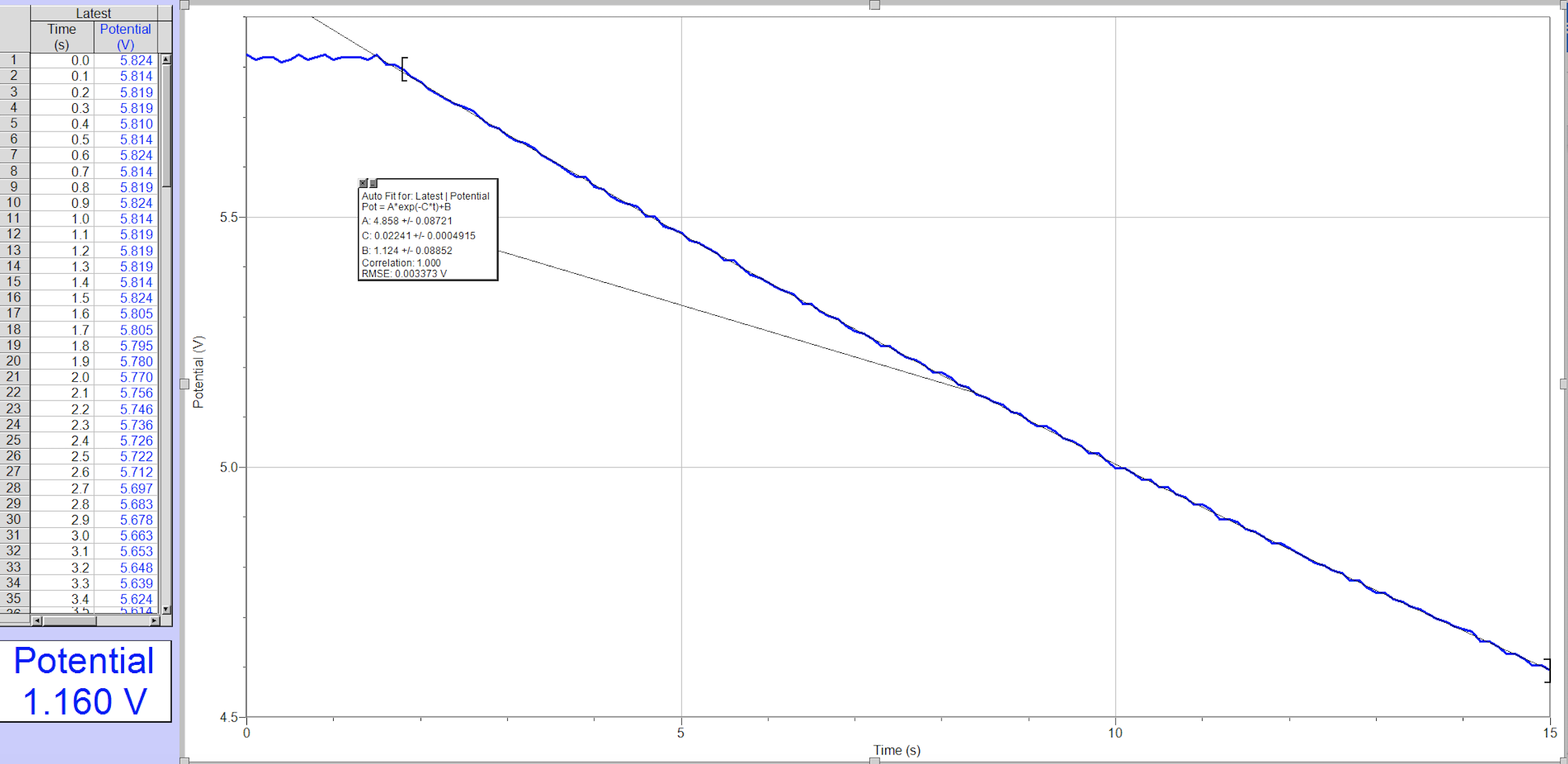
DATA TABLE Fit Parameters Resistor Capacitor Time constant Trial A B C 1/C R (Q2) C (F) RC (s) Discharge 5.771 0.851 0.0215 1/0.0215 100-KQ = 47 UF = 100,000 Q * 9 8 8 = 100,000 0.000047 F 0.000047 F = 44.340 4.7s Charge 1 15.62 -6.563 0.0822 1/0.0822 100-KQ= 47 UF = 100,000 Q* 2 2 = 100,000 0.000047 F 0.000047 F = 12.162 4.7s Discharge 4.858 1.124 0.0224 1/0.0224 47-KQ= 47 UF = 47,000 Q* 2 1 = 47,000 Q |0.000047 F 0.000047 F = 44.623 2.2s Charge 2 11.54 -5.737 0.3982 1/0.3982 47-KQ= 47 UF = 47,000 Q* 0 = 2.511 47,000 Q 0.000047 F 0.000047 F = 2.2sPROCEDURE 1. Connect the circuit as shown in Figure 1 above with the IO-uF capacitor and the 100-k resistor. Record the values of your resistor and capacitor in your data table, as well as any tolerance values marked on them. 2. Connect the Voltage Probe to the ULI and across the capacitor, with the red (positive lead) to the side of the capacitor connected to the resistor. Connect the black lead to the other side of the capacitor. 3. Prepare the computer for data collection by opening \"Exp 27\" from the Physics with Computers experiment les of Logger Pro. A graph will be displayed. The vertical axis of the graph has potential scaled from 0 to 4 V. The horizontal axis has time scaled from O to 10 s. 4. Charge the capacitor for 30 s or so with the switch 1n the position as illustrated 1n Figure 1. You can watch the voltage reading at the bottom of the screen to see if the potential" 1s still increasing. Wait until the potential 1s constant. 5 . Click to begin data collection. As soon as graphing starts, throw the switch to its other position to discharge the capacitor. Your data should show a constant value initially, then decreasing function. 6. To compare your data to the model, select only the data after the potential has started to decrease by dragging across the graph; that' 1s, omit the constant portion. Click the curve t tool E, and from the function selection box, choose the Natural Exponential function, A*exp(C*x ) + B. Click TWP\" ,and inspect the t. Clickm _ Ito return to the main graph window. '7. Record the value of the t parameters in your data table. Notice that the C used in the curve t is not the same as the C used to stand for capacitance. Compare the fit equation to the mathematical model for a capacitor discharge proposed in the introduction, 11(1) = VoleZ\"? How is t constant C related to the time constant of the circuit, which was dened in the introduction? 10. 11. 12. 13. . Print or sketch the graph of potential vs. time. Choose Store Latest Run from the Data menu to store your data. You will need this data for later analysis. The capacitor is now discharged. To monitor the charging process, click _. As soon as data collection begins, throw the switch the other way. Allow the data collection to run to completion. This time you will compare your data to the mathematical model for a capacitor charging, V0) = V,[1 e'w Select the data beginning aer the potential has started to increase by dragging across the graph. Click the curve t tool, E and from the function selection box, choose the Inverse Exponential function, A*(1 exp(C *x)) + B. Chck and inspect the t. Click@ to return to the main graph window. Record the value of the t parameters in your data table. Compare the fit equation to the mathematical model for a charging capacitor. Hide your rst runs by choosing Hide Run V Run 1 from the Data menu. Remove any remaining t information by clicking the gray close box in the oating boxes. Now you will repeat the experiment with a resistor of lower value. How do you think this change will affect the way the capacitor discharges? Rebuild your circuit using the 47-h!) resistor and repeat Steps 4 11. Capacitors The charge q on a capacitor' s plate is proportional to the potential difference V across the capacitor. We express this with V=i, C where C is a proportionality constant known as the capacitance. C is measured in the unit of the farad,F, (l farad = l coulombtvolt). If a capacitor of capacitance C (in farads), initially charged to a potential V0 (volts) is connected across a resistor R (in ohms), a time-dependent current will ow according to Ohm's law. This situation is shown by the RC (resistor-capacitor) circuit below when the switch is closed. Figure I As the current ows, the charge q is depleted, reducing the potential across the capacitor, which in turn reduces the current. This process creates an exponentially decreasing current, modeled by vm=%{%. The rate of the decrease is determined by the product RC, known as the time constant of the circuit. A large time constant means that the capacitor will discharge slowly. When the capacitor is charged, the potential across it approaches the nal value exponentially, modeled by V0)=w{1e7$). The same time constant RC describes the rate of charging as well as the rate of discharging. OBJECTIVES a Measure an experimental time constant of a resistor-capacitor circuit. a Compare the time constant to the value predicted from the component values of the resistance and capacitance. a Measure the potential across a capacitor as a function of time as it discharges and as it charges. a Fit an exponential function to the data. One of the t parameters corresponds to an experimental time constant. Latest Time Potential (S) (V) 0.0 5.824 0.1 5.814 0.2 5.819 0.3 5.819 0.4 5.810 0.5 5.814 0.6 5.824 0.7 5.814 0.8 5.819 Auto Fit for: Latest | Potential 10 0.9 5.824 Pot = A*exp(-C*t)+B 11 1.0 5.814 5.5- A: 4.858 +/- 0.08721 12 1.1 5.819 C: 0.02241+/- 0.0004915 13 1.2 5.819 B: 1.124 +/- 0.08852 14 1.3 5.819 Correlation: 1.000 RMSE: 0.003373 V 15 1.4 5.814 16 1.5 5.824 17 1.6 5.805 18 1.7 5.805 19 1.8 5.795 20 1.9 5.780 Potential (V) 21 2.0 5.770 22 2.1 5.756 23 2.2 5.746 24 2.3 5.736 25 2.4 5.726 26 2.5 5.722 27 2.6 5.712 5.0- 28 2.7 5.697 29 2.8 5.683 30 2.9 5.678 31 3.0 5.663 32 3.1 5.653 33 3.2 5.648 34 3.3 5.639 35 3.4 5.624 5614 Potential 1. 160 V 4.5- 10 15 Time (s)