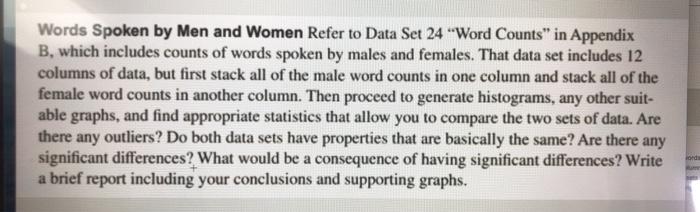
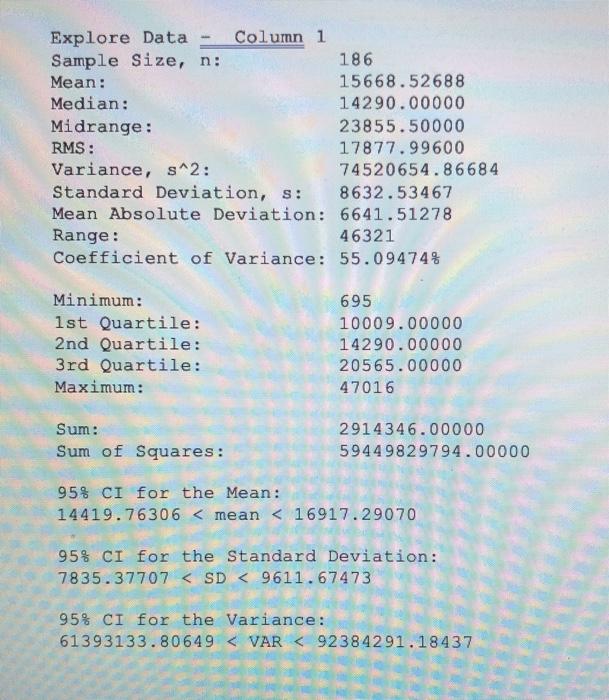
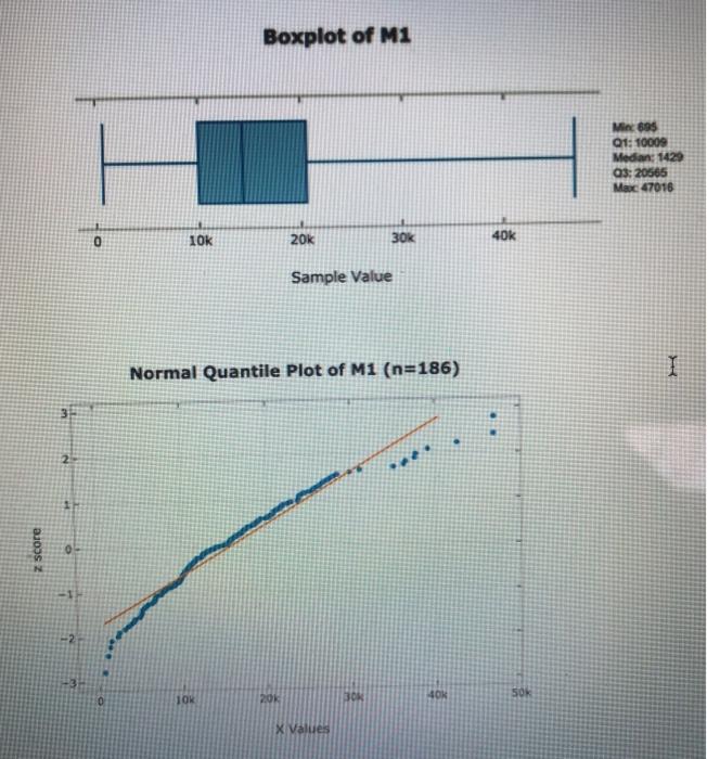
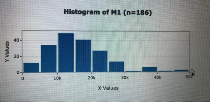
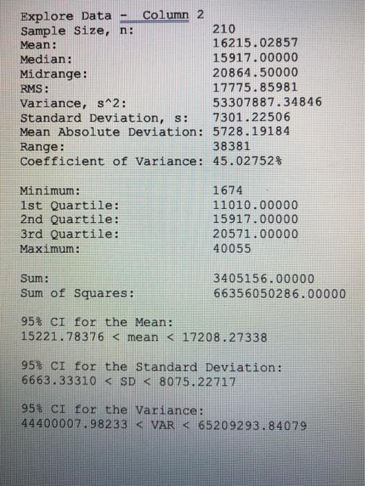
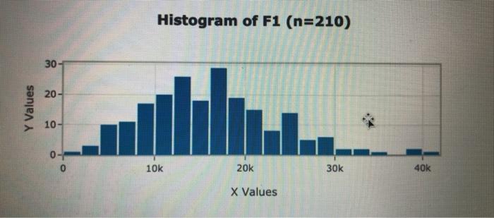
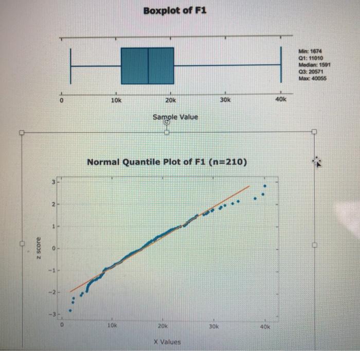
Words Spoken by Men and Women Refer to Data Set 24 "Word Counts" in Appendix B, which includes counts of words spoken by males and females. That data set includes 12 columns of data, but first stack all of the male word counts in one column and stack all of the female word counts in another column. Then proceed to generate histograms, any other suit- able graphs, and find appropriate statistics that allow you to compare the two sets of data. Are there any outliers? Do both data sets have properties that are basically the same? Are there any significant differences? What would be a consequence of having significant differences? Write a brief report including your conclusions and supporting graphs. lords Explore Data Sample Size, n: Mean: Median: Midrange: RMS: Variance, s^2: Standard Deviation, s: 8632.53467 Mean Absolute Deviation: 6641.51278 Range: Minimum: 1st Quartile: 2nd Quartile: 3rd Quartile: Maximum: Column 1 Sum: Sum of Squares: 186 46321 Coefficient of Variance: 55.09474% 15668.52688 14290.00000 23855.50000 17877.99600 74520654.86684 695 10009.00000 14290.00000 20565.00000 47016 2914346.00000 59449829794.00000 95% CI for the Mean: 14419.76306 < mean < 16917.29070 95% CI for the Standard Deviation: 7835.37707 z score 2 0 -11 -2 -3 0 10k Boxplot of M1 10k 20k Normal Quantile Plot of M1 (n=186) 20k Sample Value Sharapan pam 30k X Values 1300 5621 40K 40k 50k Min: 695 Q1:10009 Medan: 1429 03:20565 Max: 47016 I Y Values 40- 20 04 0 10k Histogram of M1 (n=186) 20k X Values 30k 40k 50 Explore Data Sample Size, n: Mean: Median: Midrange: RMS: Variance, s^2: Standard Deviation, s: Mean Absolute Deviation: Range: Coefficient of Variance: had Minimum: 1st Quartile: 2nd Quartile: 3rd Quartile: Maximum: Column 2 Sum: Sum of Squares: 210 16215.02857 15917.00000 20864.50000 17775.85981 53307887.34846 7301.22506 5728.19184 38381 45.02752% 1674 11010.00000 15917.00000 20571.00000 40055 3405156.00000 66356050286.00000 95% CI for the Mean: 15221.78376 < mean < 17208.27338 95% CI for the Standard Deviation: 6663.33310 Y Values 30 20- 10 Histogram of F1 (n=210) 10k 20k X Values 30k 40k z score N 0 10k Boxplot of F1 10k 20k Sample Value Normal Quantile Plot of F1 (n=210) 20k X Values 30k 30k 40k 40k Min: 1674 Q1: 11010 Median: 1591 Q3: 20571 Max 40055