Write a computer program that performs the procedure described in Example 4.2 in the textbook. Use the results of running your program to make figures that are equivalent to Fig 4.8(c) and (d) in the textbook. Make sure to show both the matrices and related histograms that show the number of sites that have Q quanta. Explain how you could use the histograms to work out the temperature of the systems.

use python ,thank you

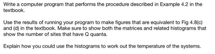
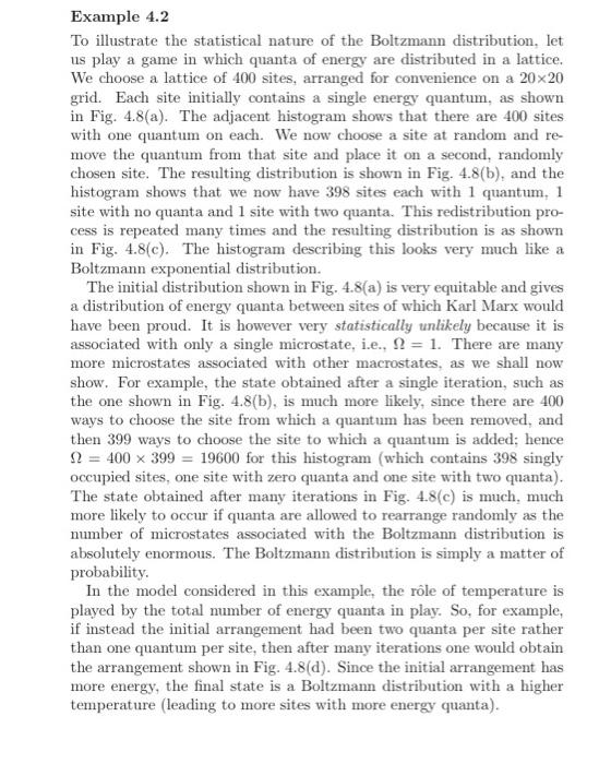
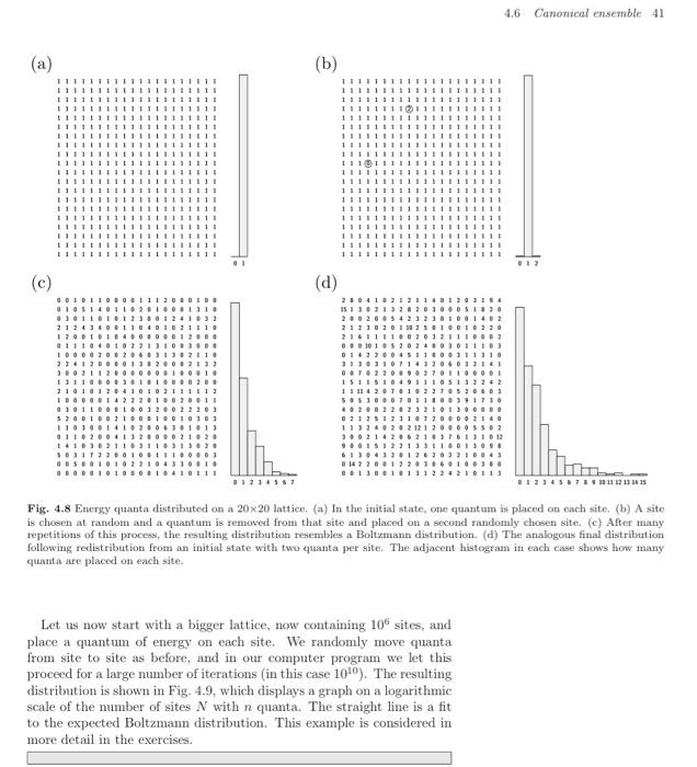
Write a computer program that performs the procedure described in Example 4.2 in the textbook. Use the results of running your program to make figures that are equivalent to Fig 4.8(c) and (d) in the textbook. Make sure to show both the matrices and related histograms that show the number of sites that have Q quanta. Explain how you could use the histograms to work out the temperature of the systems. Example 4.2 To illustrate the statistical nature of the Boltzmann distribution, let us play a game in which quanta of energy are distributed in a lattice. We choose a lattice of 400 sites, arranged for convenience on a 20x20 grid. Each site initially contains a single energy quantum, as shown in Fig. 4.8(a). The adjacent histogram shows that there are 400 sites with one quantum on each. We now choose a site at random and re- move the quantum from that site and place it on a second, randomly chosen site. The resulting distribution is shown in Fig. 4.8(b), and the histogram shows that we now have 398 sites each with 1 quantum, 1 site with no quanta and 1 site with two quanta. This redistribution pro- cess is repeated many times and the resulting distribution is as shown in Fig. 4.8(c). The histogram describing this looks very much like a Boltzmann exponential distribution. The initial distribution shown in Fig. 4.8(a) is very equitable and gives a distribution of energy quanta between sites of which Karl Marx would have been proud. It is however very statistically unlikely because it is associated with only a single microstate, i.e., 9 = 1. There are many more microstates associated with other macrostates, as we shall now show. For example, the state obtained after a single iteration, such as the one shown in Fig. 4.8(b), is much more likely, since there are 400 ways to choose the site from which a quantum has been removed, and then 399 ways to choose the site to which a quantum is added: hence A = 400 x 399 = 19600 for this histogram (which contains 398 singly occupied sites, one site with zero quanta and one site with two quanta). The state obtained after many iterations in Fig. 4.8(e) is much, much more likely to occur if quanta are allowed to rearrange randomly as the number of microstates associated with the Boltzmann distribution is absolutely enormous. The Boltzmann distribution is simply a matter of probability. In the model considered in this example, the role of temperature is played by the total number of energy quanta in play. So, for example, if instead the initial arrangement had been two quanta per site rather than one quantum per site, then after many iterations one would obtain the arrangement shown in Fig. 4.8(d). Since the initial arrangement has more energy, the final state is a Boltzmann distribution with a higher temperature (leading to more sites with more energy quanta). 4.6 Canonical ensemble 41 (a) (b) ) 11111 !!!!!111011 111111111 11111 111 (c) (d) 11241 IPO! 111 7101 113.21 2020.3 211102013 211111 ...151 0173 313310 151151 SUIS 1112 5.1 4.. 21 1512111311.01 13.12.2011 014 17.3...11 6.1.1.11123) .123.58 012345.711211215315 Fig. 4.8 Energy quanta distributed on a 20x20 lattice. (a) In the initial state, one quantum is placed on each site. (b) A site is chosen at random and a quantum is removed from that site and placed on a second randomly chosen site. (c) After many repetitions of this process, the resulting distribution resembles a Boltzmann distribution. (d) The analogous final distribution following redistribution from an initial state with two quanta per site. The adjacent histogram in each case shows how many quanta are placed on each site. Let us now start with a bigger lattice, now containing 106 sites, and place a quantum of energy on each site. We randomly move quanta from site to site as before, and in our computer program we let this proceed for a large number of iterations (in this case 1010). The resulting distribution is shown in Fig. 4.9, which displays a graph on a logarithmic scale of the number of sites N with n quanta. The straight line is a fit to the expected Boltzmann distribution. This example is considered in more detail in the exercises. a