Write a MATLAB code that solves the 1-D Heat Equation in using explicit, implicit and crank-nicholson methods.

I'm having issues writing the initial conditions and I would appreciate any help on this.

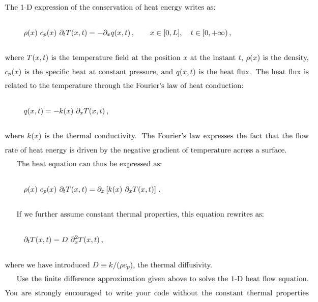
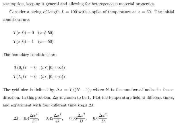
The 1-D expression of the conservation of heat energy writes as: P(T) cp(T) 0T (, t)= -0,q(z, t), (0,1), t[0, +00), where T' (2, ) is the temperature field at the position r at the instant t, p(x) is the density, p(1) is the specific heat at constant pressure, and qx, t) is the heat flux. The heat flux is related to the temperature through the Fourier's law of heat conduction: qr,t)=-k(2) 8,72,1), where k(r) is the thermal conductivity. The Fourier's law expresses the fact that the flow rate of heat energy is driven by the negative gradient of temperature across a surface. The heat equation can thus be expressed as: p(1) Gp() @T(1,t) = 0,[k() ,T(3,4)) If we further assume constant thermal properties, this equation rewrites as: @T(1,t) = D 2T(z,t), where we have introduced D= k/(pop), the thermal diffusivity. Use the finite difference approximation given above to solve the 1-D heat flow equation. You are strongly encouraged to write your code without the constant thermal properties assumption, keeping it general and allowing for heterogeneous material properties. Consider a string of length L = 100 with a spike of temperature at r = 50. The initial conditions are: T(3,0) = 0 ( 250) T(1,0)=1 (1 = 50) The boundary conditions are: T(0,t) = 0 (te [0,+)) T(L,t) = 0 (te [0, +0) The grid size is defined by Az = L/(N 1), where N is the number of nodes in the x- direction. In this problem, Ar is chosen to be 1. Plot the temperature field at different times, and experiment with four different time steps At: Ara At = 0.4 D z2 0.45 D A..? 0.55 D Aca 0.6 D 3 9 The 1-D expression of the conservation of heat energy writes as: P(T) cp(T) 0T (, t)= -0,q(z, t), (0,1), t[0, +00), where T' (2, ) is the temperature field at the position r at the instant t, p(x) is the density, p(1) is the specific heat at constant pressure, and qx, t) is the heat flux. The heat flux is related to the temperature through the Fourier's law of heat conduction: qr,t)=-k(2) 8,72,1), where k(r) is the thermal conductivity. The Fourier's law expresses the fact that the flow rate of heat energy is driven by the negative gradient of temperature across a surface. The heat equation can thus be expressed as: p(1) Gp() @T(1,t) = 0,[k() ,T(3,4)) If we further assume constant thermal properties, this equation rewrites as: @T(1,t) = D 2T(z,t), where we have introduced D= k/(pop), the thermal diffusivity. Use the finite difference approximation given above to solve the 1-D heat flow equation. You are strongly encouraged to write your code without the constant thermal properties assumption, keeping it general and allowing for heterogeneous material properties. Consider a string of length L = 100 with a spike of temperature at r = 50. The initial conditions are: T(3,0) = 0 ( 250) T(1,0)=1 (1 = 50) The boundary conditions are: T(0,t) = 0 (te [0,+)) T(L,t) = 0 (te [0, +0) The grid size is defined by Az = L/(N 1), where N is the number of nodes in the x- direction. In this problem, Ar is chosen to be 1. Plot the temperature field at different times, and experiment with four different time steps At: Ara At = 0.4 D z2 0.45 D A..? 0.55 D Aca 0.6 D 3 9