

Question: write a more efficient version of the function called poly _ opt that takes the same parameters in the same order and returns the same
write a more efficient version of the function called polyopt that takes the same parameters in the same order and returns the same result. double polyoptdouble adouble x long degree
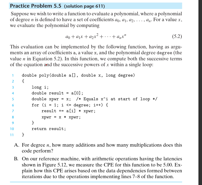
Practice Problem solution page
Suppose we wish to write a function to evaluate a polynomial, where a polynomial of degree n is defined to have a set of coefficients a a aldots an For a value x we evaluate the polynomial by computing
aa xa xcdotsan xn
This evaluation can be implemented by the following function, having as arguments an array of coefficients a a value x and the polynomial degree degree the value n in Equation In this function, we compute both the successive terms of the equation and the successive powers of x within a single loop:
double polydouble a double x long degree
long i;
double result a;
double xpwr x; Equals xi at start of loop
for i ; i degree; i
result ai xpwr;
xpwr x xpwr;
return result;
A For degree n how many additions and how many multiplications does this code perform?
B On our reference machine, with arithmetic operations having the latencies shown in Figure we measure the CPE for this function to be Explain how this CPE arises based on the data dependencies formed between iterations due to the operations implementing lines of the function. Practice Problem solution page
Let us continue exploring ways to evaluate polynomials, as described in Practice Problem We can reduce the number of multiplications in evaluating a polynomial by applying Horner's method, named after British mathematician William G Horner The idea is to repeatedly factor out the powers of x to get the following evaluation:
axleftaxleftacdotsxleftanx anrightcdotsrightright
Using Horner's method, we can implement polynomial evaluation using the following code:
Apply Horner's method
double polyhdouble a double x long degree
long i;
double result adegree;
for i degree; i ; i
result ai xresult;
return result;
A For degree n how many additions and how many multiplications does this code perform?
B On our reference machine, with the arithmetic operations having the latencies shown in Figure we measure the CPE for this function to be Explain how this CPE arises based on the data dependencies formed between iterations due to the operations implementing line of the function.
C Explain how the function shown in Practice Problem can run faster, even though it requires more operations. Practice Problem solution page
Suppose we wish to write a function to evaluate a polynomial, where a polynomial of degree n is defined to have a set of coefficients a a aldots an For a value x we evaluate the polynomial by computing
aa xa xcdotsan xn
This evaluation can be implemented by the following function, having as arguments an array of coefficients a a value x and the polynomial degree degree the value n in Equation In this function, we compute both the successive terms of the equation and the successive powers of x within a single loop:
double polydouble a double x long degree
long i;
double result a;
double xpwr x; Equals xi at start of loop
for i ; i degree; i
result ai xpwr;
xpwr x xpwr;
return result;
A For degree n how many additions and how many multiplications does this code perform?
B On our reference machine, with arithmetic operations having the latencies shown in Figure we measure the CPE for this function to be Explain how this CPE arises based on the data dependencies formed between iterations due to the operations implementing lines of the function. Practice Problem solution page
Let us continue exploring ways to evaluate polynomials, as described in Practice Problem We can reduce the number of multiplications in evaluating a polynomial by applying Horner's method, named after British mathematician William G Horner The idea is to repeatedly factor out the powers of x to get the following evaluation:
axleftaxleftacdotsxleftanx anrightcdotsrightright
Using Horner's method, we can implement polynomial evaluation using the following code:
Apply Horner's method
double polyhdouble a double x long degree
long i;
double result adegree;
for i degree; i ; i
result ai xresult;
return result;
A For degree n how many additions and how many multiplications does this code perform?
B On our reference machine, with the arithmetic operations having the lat
Step by Step Solution
There are 3 Steps involved in it
1 Expert Approved Answer
Step: 1 Unlock

Question Has Been Solved by an Expert!
Get step-by-step solutions from verified subject matter experts
Step: 2 Unlock
Step: 3 Unlock