Write a python program on jupyter notebook implementing the Black Scholes Equation. The input values should be :

S= 100 (spot price)

K = 30 (strike price)

r = 0.05 (rate)

sigma = 0.2 (volatility)

T = 2 (time interval)

M = 100

N = 100

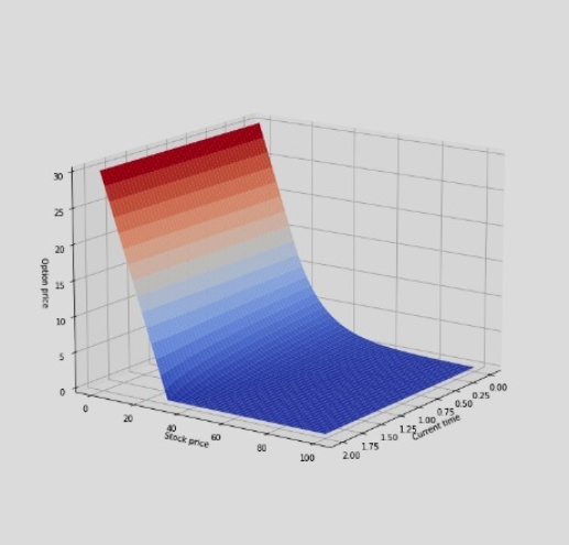
The below mentioned code is incorrect. You can use it for reference and edit it however you please. If done corectly, the output should be this :

My current code is completely wrong i think and this is the resultant output :

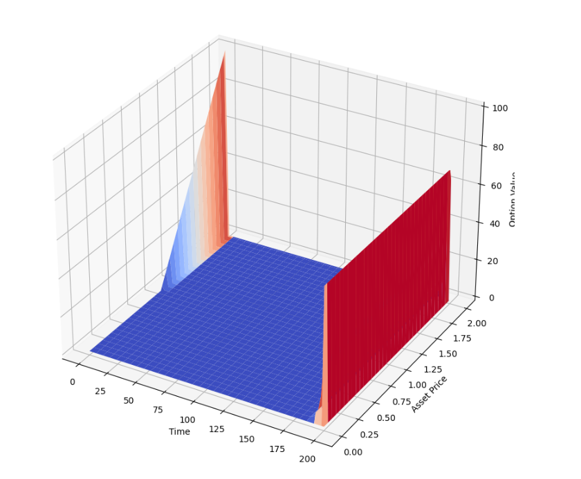
Please do the necessary changes and correct it to match the exact output given above

import numpy as np from scipy.optimize import fsolve from scipy.interpolate import interp2d from typing import Callable #Implementing the use of a class to solve the BSM PDE using the implicit finite difference scheme. class BSMPDESolver: def __init__(self, spot_price, strike_price, maturity, volatility, interest_rate, dividend_yield, payoff_function: Callable): self.S = spot_price self.K = strike_price self.T = maturity self.sigma = volatility self.r = interest_rate self.q = dividend_yield self.payoff_function = payoff_function def solve_pde(self, option_type='European', grid_size=(100, 100)): M, N = grid_size dt = self.T / M dS = (2 * self.S) / N # Initialize grid S_values = np.linspace(0, 2 * self.S, N + 1) t_values = np.linspace(0, self.T, M + 1) grid = np.zeros((M + 1, N + 1)) # Set boundary conditions grid[:, 0] = self.payoff_function(S_values) grid[:, -1] = 0 if option_type == 'European' else self.K - S_values[-1] # Solve the implicit finite difference scheme for i in range(M - 1, 0, -1): A = self._build_coefficient_matrix(grid[i + 1, 1:-1], dS, dt) B = self._build_rhs_vector(grid[i + 1, 1:-1], dS, dt, S_values[1:-1], t_values[i]) grid[i, 1:-1] = fsolve(lambda x: np.dot(A, x) - B, grid[i, 1:-1]) return S_values, t_values, grid def _build_coefficient_matrix(self, u_next, dS, dt): sigma2 = self.sigma**2 r = self.r q = self.q alpha = 0.5 * dt * (sigma2 * np.arange(1, len(u_next) + 1)**2 - (r - q) * np.arange(1, len(u_next) + 1)) beta = 1 + dt * (sigma2 * np.arange(1, len(u_next) + 1)**2 + r) gamma = -0.5 * dt * (sigma2 * np.arange(1, len(u_next) + 1)**2 + (r - q) * np.arange(1, len(u_next) + 1)) A = np.diag(alpha[:-1], -1) + np.diag(beta) + np.diag(gamma[:-1], 1) return A def _build_rhs_vector(self, u_next, dS, dt, S_values, t): sigma2 = self.sigma**2 r = self.r q = self.q b = u_next.copy() b[0] -= 0.5 * dt * (sigma2 * 1**2 - (r - q) * 1) * (self.payoff_function(S_values[0]) - self.payoff_function(S_values[0] - dS)) b[-1] -= 0.5 * dt * (sigma2 * len(u_next)**2 + (r - q) * len(u_next)) * (self.K - S_values[-1]) return b # Sample question : if __name__ == "__main__": def payoff_function(S): return np.maximum(0, S - 100) # Example payoff function (call option) bsm_solver = BSMPDESolver(spot_price=100, strike_price=30, maturity=2, volatility=0.2, interest_rate=0.05, dividend_yield=0.02, payoff_function=payoff_function) S_values, t_values, option_prices = bsm_solver.solve_pde() # Print or visualize the results as needed print(option_prices)import matplotlib.pyplot as plt from mpl_toolkits.mplot3d import Axes3D # Assuming option_prices is the result from your PDE solver fig = plt.figure(figsize=(10, 10)) ax = fig.add_subplot(111, projection='3d') X, Y = np.meshgrid(S_values, t_values) Z=option_prices ax.plot_surface(X, Y, Z, cmap='coolwarm') ax.set_xlabel('Time') ax.set_ylabel('Asset Price') ax.set_zlabel('Option Value') ax.set_title('Option Value Surface Plot') plt.show()

NOTE : Kindly run your outputs on Jupyter Notebook before posting your answer as I have received wrong answers multiple times.

2