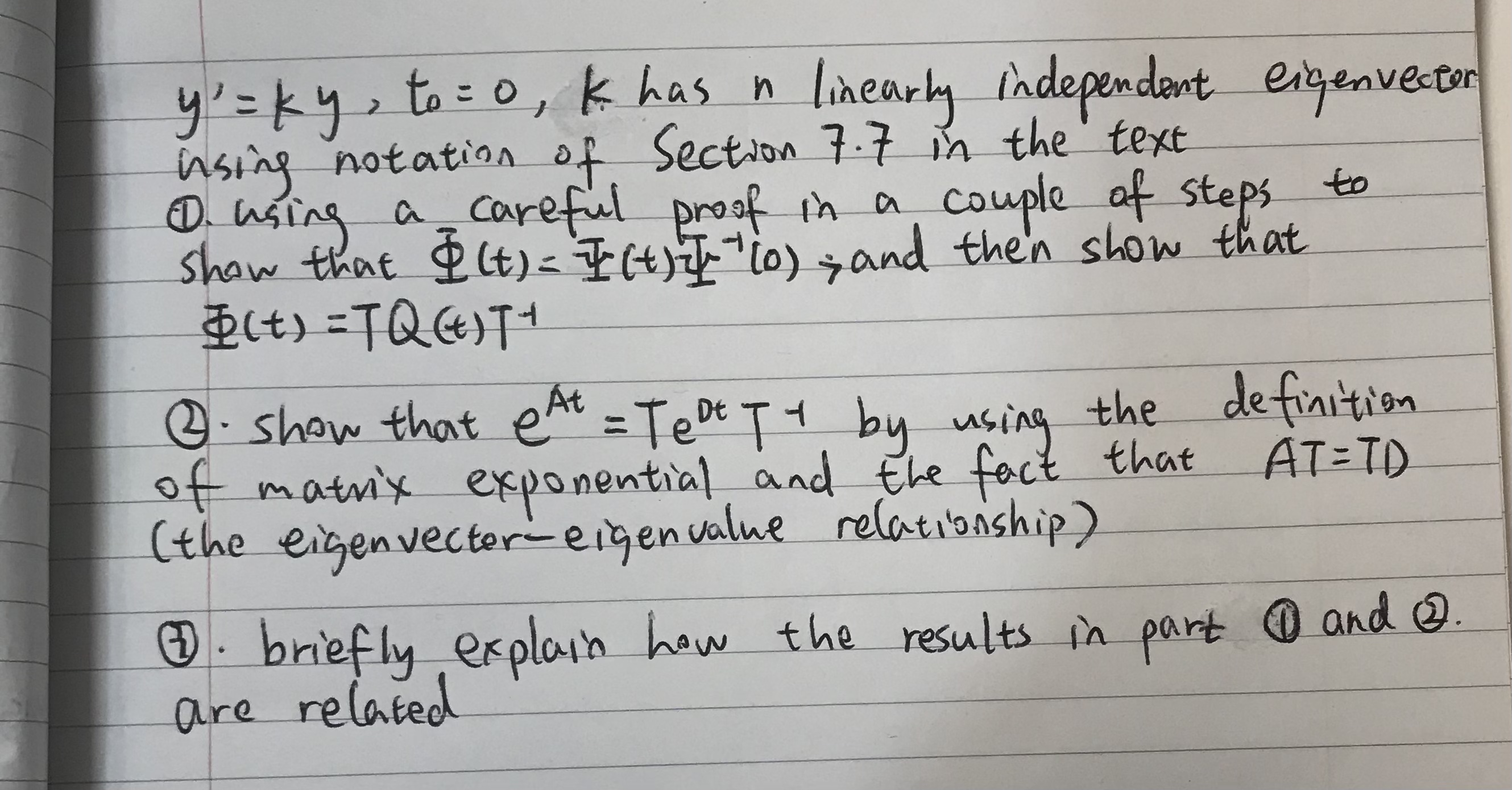
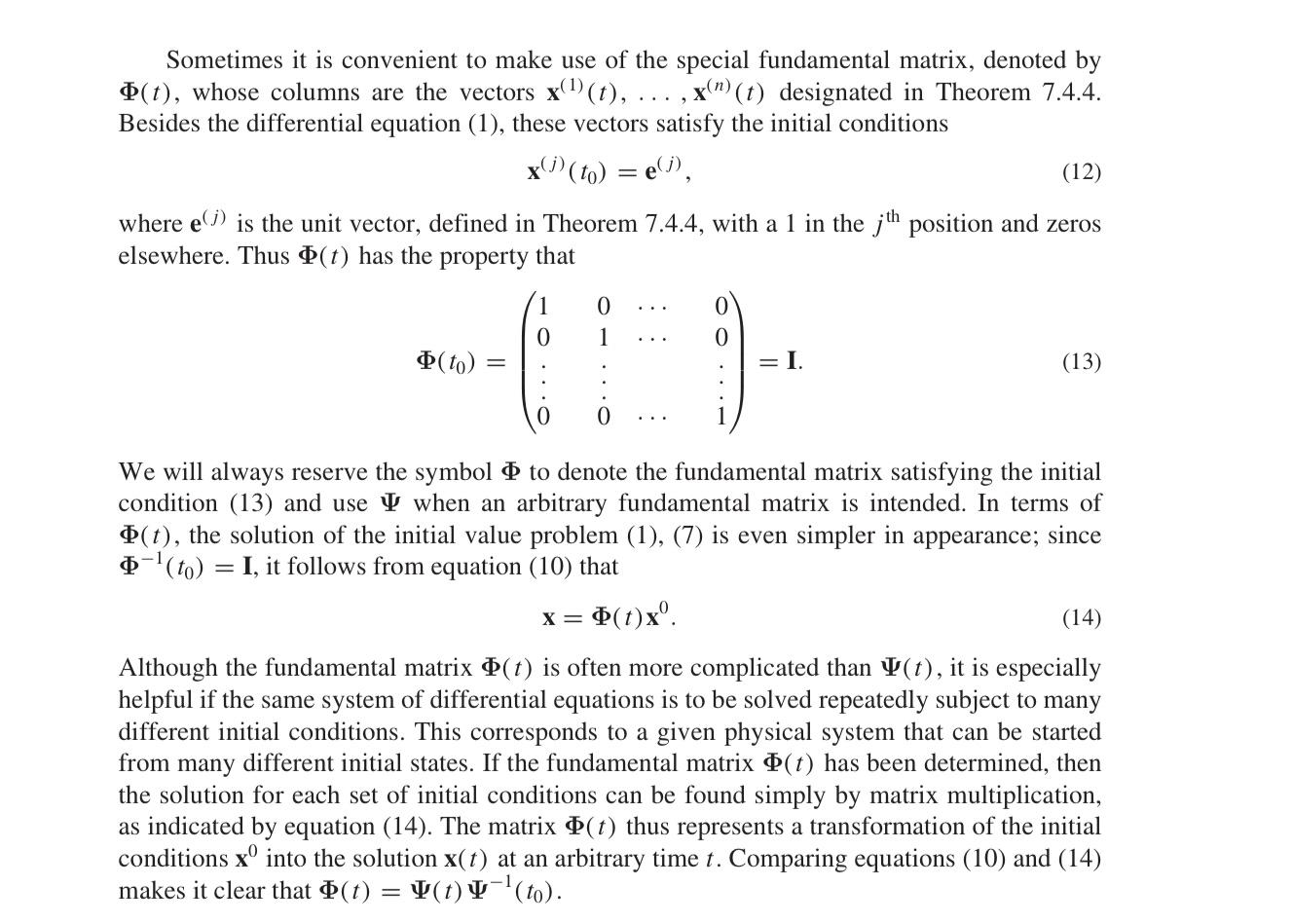
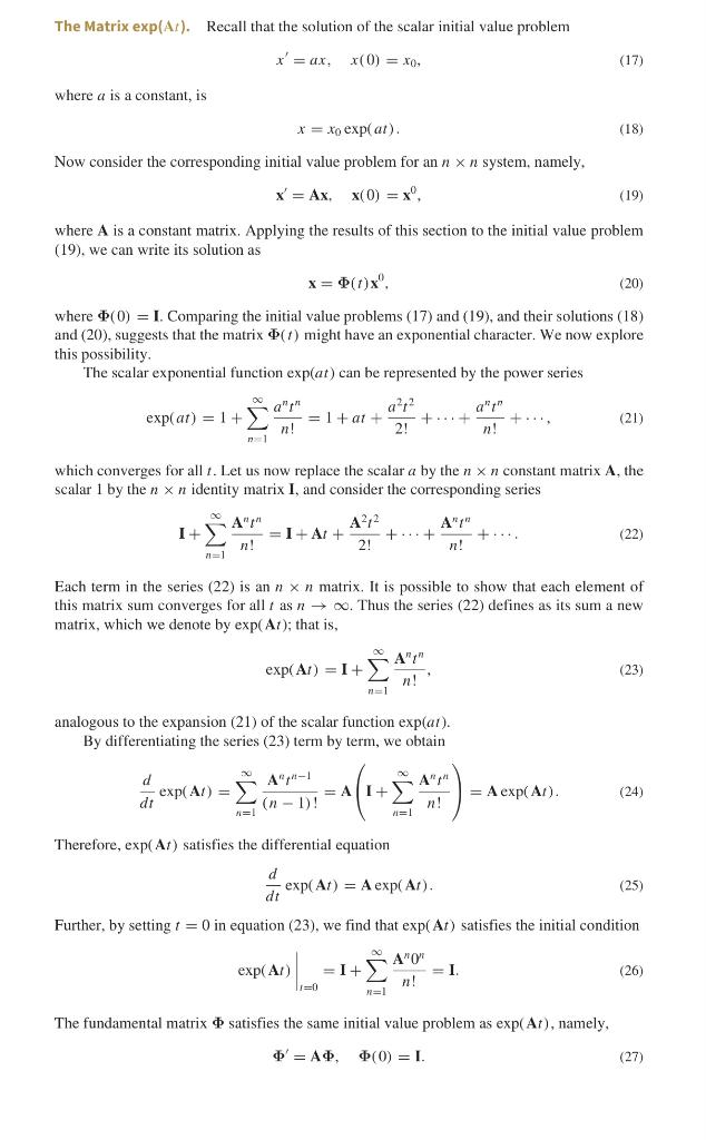
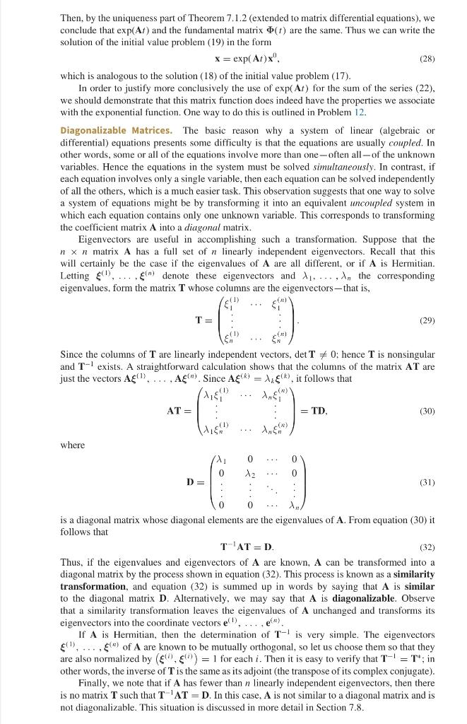
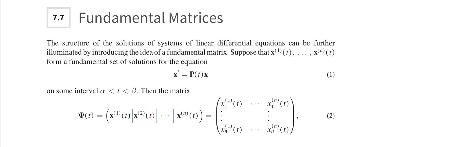
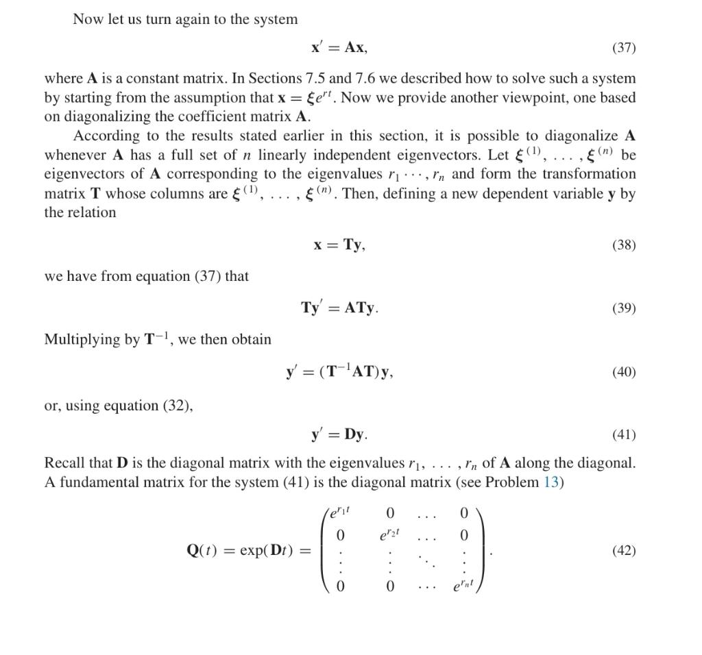
y' = ky , to = 0, k has n linearly independent eigenvector insing notation of Section 7.7 in the text D. using a careful proof in a couple of steps to show that P ( t) = I (t) T 10) , and then show that B (+ ) = TQ ( + ) T + show that pat = Tent 1 by using the definition of matrix exponential and the fact that AT = TD ( the eigenvector - eigenvalue relationship ) J. briefly explain how the results in part and @ are relatedSometimes it is convenient to make use of the special fundamental matrix, denoted by CPU), whose columns are the vectors x(\"(t), .. . ,x(")(t) designated in Theorem 7.4.4. Besides the differential equation (1), these vectors satisfy the initial conditions x'j'm) = e\"), (12) where em is the unit vector, defined in Theorem 7.4.4, with a 1 in the j \"1 position and zeros elsewhere. Thus (EU) has the property that l O 0 0 1 0 (1 (1 i We will always reserve the symbol '1' to denote the fundamental matrix satisfying the initial condition (13) and use '1' when an arbitrary fundamental matrix is intended. In terms of @(t), the solution of the initial value problem (1), (7) is even simpler in appearance; since @400) = I, it follows from equation (10) that x = qa(r)x. (14) Although the fundamental matrix @( t) is often more complicated than l1'( 1') , it is especially helpful if the same system of differential equations is to be solved repeatedly subject to many different initial conditions. This corresponds to a given physical system that can be started from many different initial states. If the fundamental matrix @(I) has been determined, then the solution for each set of initial conditions can be found simply by matrix multiplication, as indicated by equation (14). The matrix (PU) thus represents a transformation of the initial conditions X\" into the solution x(t) at an arbitrary time t. Comparing equations (10) and (14) makes it clear that @(t) = \\Il(t)\\I"1(rg). The Matrix exp(Ar). Recall that the solution of the scalar initial value problem x = ax, x(0) = x0, (17) where a is a constant, is x = xo exp( at) . (18) Now consider the corresponding initial value problem for an n x n system, namely. X' = Ax, x(0) = x", (19) where A is a constant matrix. Applying the results of this section to the initial value problem (19). we can write its solution as x = $(1)x". (20) where (0) = I. Comparing the initial value problems (17) and (19), and their solutions (18) and (20), suggests that the matrix (/) might have an exponential character. We now explore this possibility. The scalar exponential function exp(ar) can be represented by the power series exp(at) = 1+ ) a-12 =1+ar+ 2! +...+ + ... (21) n! which converges for all f. Let us now replace the scalar a by the n X n constant matrix A, the scalar 1 by the n x n identity matrix I, and consider the corresponding series I+ A272 = I+ Ar + 2! +.. + n! +.... (22) 71=1 n! Each term in the series (22) is an n x n matrix. It is possible to show that each element of this matrix sum converges for all f as n -> co. Thus the series (22) defines as its sum a new matrix, which we denote by exp( At ); that is, exp(A!) = 1+ ) n ! (23) analogous to the expansion (21) of the scalar function exp(ar ). By differentiating the series (23) term by term, we obtain - exp( A/) = ) Art#-1 (n - 1) ! = A I+ n ! = A exp( Ar). (24) M=1 1=1 Therefore, exp( Ar) satisfies the differential equation d dt - exp( At) = A exp( Ar). (25) Further, by setting / = 0 in equation (23), we find that exp( Ar) satisfies the initial condition exp( Ar) =1+ A"()" =1. (26) 1=0 n=1 n! The fundamental matrix + satisfies the same initial value problem as exp( Ar), namely, D' = Ad, $(0) =1. (27)Then, by the uniqueness part of Theorem 7.1.2 [extended to matrix differential equations}1 we conclude that expthtl and the fundamental matrix in\") are the same. Thus we can write the solution of the initial value problem (19} in the form x = expanx\". (23) which is analogous to the solution {18} of the initial value problem [11}. In order to justify more conclusively the use of espt Al} for the sum of the series [22}, we should demonstrate that this matrix function does indeed have the properties we associate with the Exponential function. One way to do this is outlined in Problem I2. Diagonalizable Matrices. The basic reason why a system of linear {algebraic or differential} equations presents some difculty is that the equations are usually coupled. in other words. some or all of the equations involve more than oneoften allol' the unknown variables. Hence the equations in the system must be solved simltmteoasly. In contrast. if each equation invtrl'ves only a single variahle, then each equation can be solved independently of all the others, which is a much easier task. This observation suggests that one way to solve a system of equations might be by transforming it into an equivalent uncoupled system in which each equation contains only one unknown variable. This corresponds to transforming the coefcient matrix a into a diagonal matrix. Eigenvectors are useful in accomplishing such a transformation. Suppose that the n x in matrix A. has a full set of a linearly independent eigenvectms. Recall that this will certainly be the case if the eigenvalues of A are all different, or if A is l-Ierrnitian. Letting E\"). .Ei'\" denote these eigenvectors and l1.,}i,. the corresponding eigenvalues. forrn the matrix T whose columns are the eigenvectorsthat is, all ginl T: 3 '- . :29: {Ill in] Fl _ Since the columns of T are linearly independent vectors. detT 5.2 l]: hence T is nonsingular and T'1 exists. A straightforward calculation shows that the columns of the matrix AT are just the vectors 3.5\"}, . .. .AE'"3'. Since NEW = Ayilit follows that l. r: is? as? err = = T1). (303' Ali-fir\" nalist where (Ill! [1 {i a s2 o n = . . _ . on o o J... is a diagonal rnalrix whose diagonal elements are the eigenvalues of A. From equation {ll} it follows that 'r"'s'r = D. (as) Thus. if the eigenvalues and eigenvectors of A. are known. A. can be transformed into a diagonal matrix by the process shown in equation t32). This process is known as a similarity transformation, and equation {32) is summed up in words by saying that A is similar to the diagonal matrix B. Alternatively, we may say that A. is diagonalinable. Observe that a similarity transformation leaves the eigenvalues of A. unchanged and transforms its eigenvectors into the coordinate vectors e' '3, . . . . 2\"\". [l A. is Hermitian. then the determination of T1 is very simple. The eigenvectors {{1'. . . . .El} of A. are known to be mutually orthogonal. so let us choose them so that they are also normalised hy {Eli}, E\") = l for each 1'. Then it is easy to verify that T" = "I\"; in other words, the inverse of T is the same as its adjoint {the transpose of its complex conjugate). Finally. we note that if s has fewer than a linearly independent eigenvectors. then there is no matrix T such that T \"1 AT = I}. In this case. A is not similar to a diagonal matrix and is not diagonalisahle. This situation is discussed in more detail in Section 1.3. 7.7 Fundamental Matrices The structure of the solutions of systems of linear differential equations can be further illuminated by introducing the idea of a fundamental matrix. Suppose that x() (t), . . . , x(") (t) form a fundamental set of solutions for the equation X = P(t) x (1) on some interval a