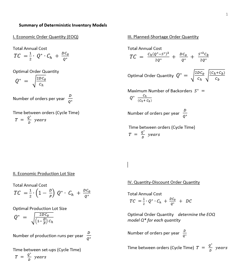
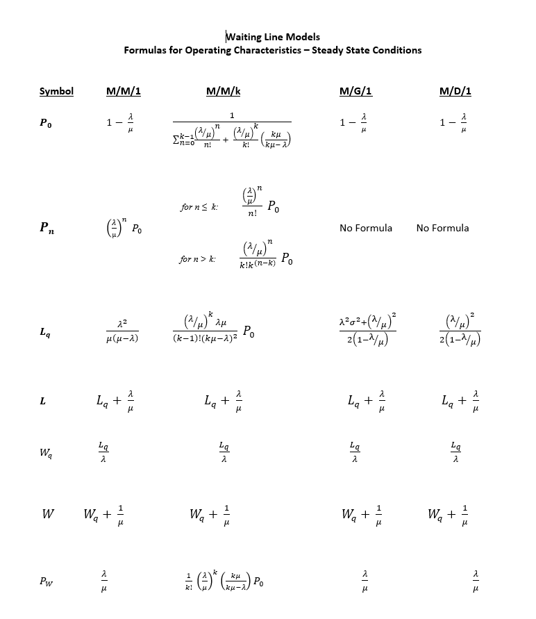
you will be developing 2 case studies. A case study requires an individual to create a simulation or realistic scenario that integrates the knowledge and skills they have acquired. Specifically, you will be using the theory and the math used in Chapter 10 on Inventory Models and Chapter 11 on Queuing Theory to develop two separate situations. Parameters: you must use all of the formulas used from Chapter 10.1 -10.6 and Chapter 11 (11.1-11.7).Because there is an element of subjectivity to this project, BE THOROUGH. As far as page count, each case study and the work following it should be a few pages.

1 Summary of Deterministic Inventory Models 1. Economic Order Quantity (EOQ) III. Planned-Shortage Order Quantity Total Annual Cost TC = Q* Cn + DCO Total Annual Cost TC Cn(Q*-s*)2 20* = + DCO Q* + S2CD 20* 2 Q* Optimal Order Quantity Q* 2D Co Ch Optimal Order Quantity Q* = 2DCa | Ch+Cb) Ch = = D Number of orders per year Maximum Number of Backorders S* Ch Q* (CA+C) Q* Number of orders per year Time between orders (Cycle Time) years Q* T = D Time between orders (Cycle Time) 2* T years = D | II. Economic Production Lot Size IV. Quantity-Discount Order Quantity Total Annual Cost TC = (1-) Q* - CH + DCO Q* Total Annual Cost 2 DCO TC = 2*.CH + + DC Q Optimal Production Lot Size 2D CO Q* (1-3/) con = Optimal Order Quantity determine the EOQ model Q* for each quantity Number of orders per year Number of production runs per year Time between orders (Cycle Time) T = q year's D Time between set-ups (Cycle Time) T = years D Waiting Line Models Formulas for Operating Characteristics - Steady State Conditions Symbol M/M/1 M/M/k M/G/1 M/D/1 1 1 - 1 1 1 k (9)". (/ 9 | | 8 sk-1 2n=0 + ku ku- n! k! for nsk: n! n PR )" Po No Formula No Formula n (1/)" for n>k: P. k!k (n-k) k La 22 (-) (2/4)" nu (k-1)!(ku-2) P. 12o2+(44) 2(1-7) (W/M) 2(1-4) a a 2 L La + La + La + La + u La a LQ wa LQ 2 2 R W W. + Wq+ 1 + 1 W. + 1 u i ku a Pw en 019* Chihetra) P. | u U 1 Summary of Deterministic Inventory Models 1. Economic Order Quantity (EOQ) III. Planned-Shortage Order Quantity Total Annual Cost TC = Q* Cn + DCO Total Annual Cost TC Cn(Q*-s*)2 20* = + DCO Q* + S2CD 20* 2 Q* Optimal Order Quantity Q* 2D Co Ch Optimal Order Quantity Q* = 2DCa | Ch+Cb) Ch = = D Number of orders per year Maximum Number of Backorders S* Ch Q* (CA+C) Q* Number of orders per year Time between orders (Cycle Time) years Q* T = D Time between orders (Cycle Time) 2* T years = D | II. Economic Production Lot Size IV. Quantity-Discount Order Quantity Total Annual Cost TC = (1-) Q* - CH + DCO Q* Total Annual Cost 2 DCO TC = 2*.CH + + DC Q Optimal Production Lot Size 2D CO Q* (1-3/) con = Optimal Order Quantity determine the EOQ model Q* for each quantity Number of orders per year Number of production runs per year Time between orders (Cycle Time) T = q year's D Time between set-ups (Cycle Time) T = years D Waiting Line Models Formulas for Operating Characteristics - Steady State Conditions Symbol M/M/1 M/M/k M/G/1 M/D/1 1 1 - 1 1 1 k (9)". (/ 9 | | 8 sk-1 2n=0 + ku ku- n! k! for nsk: n! n PR )" Po No Formula No Formula n (1/)" for n>k: P. k!k (n-k) k La 22 (-) (2/4)" nu (k-1)!(ku-2) P. 12o2+(44) 2(1-7) (W/M) 2(1-4) a a 2 L La + La + La + La + u La a LQ wa LQ 2 2 R W W. + Wq+ 1 + 1 W. + 1 u i ku a Pw en 019* Chihetra) P. | u U