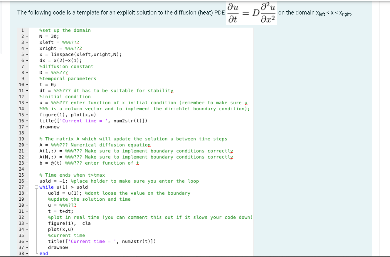
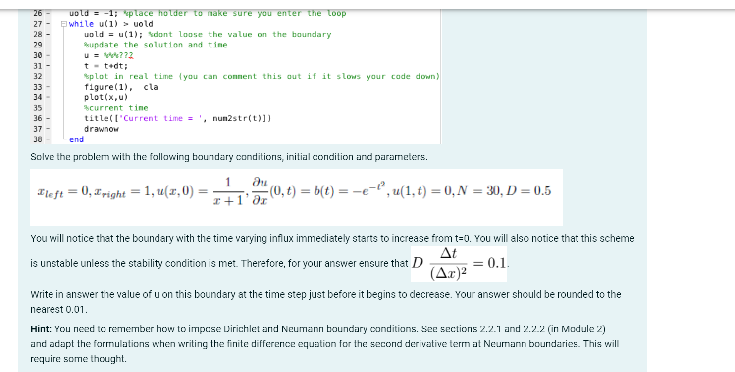
zu The following code is a template for an explicit solution to the diffusion (heat) PDE on the domain Xleft tmax uold = -1; $place holder to make sure you enter the loop while u(1) > uold uold = u(1); %dont loose the value on the boundary %update the solution and time u = %%%??? t = tudt; %plot in real time (you can comment this out if it slows your code down) figure(1), cla plot(x,u) $current time title(['Current time = " num2 str(t)]) drawnow end 26 27 28 29 30 31 32 33 34 35 36 37 38 uold = -1; *place holder to make sure you enter the loop while u(1) > uold uold = u(1); %dont loose the value on the boundary %update the solution and time u = %%%??? t = tudt; Splot in real time (you can comment this out if it slows your code down) figure(1), cla plot(x,u) %current time title(['Current time = num2 str(t))) drawnow end Solve the problem with the following boundary conditions, initial condition and parameters. 1 Ileft = 0, Bright = 1, u(2,0) au (0,t) = b(t) = -e-, u(1, t) = 0, N = 30, D=0.5 2+1' ar You will notice that the boundary with the time varying influx immediately starts to increase from t=0. You will also notice that this scheme At is unstable unless the stability condition is met. Therefore, for your answer ensure that D = 0.1. (A.x)2 Write in answer the value of u on this boundary at the time step just before it begins to decrease. Your answer should be rounded to the nearest 0.01. Hint: You need to remember how to impose Dirichlet and Neumann boundary conditions. See sections 2.2.1 and 2.2.2 (in Module 2) and adapt the formulations when writing the finite difference equation for the second derivative term at Neumann boundaries. This will require some thought. zu The following code is a template for an explicit solution to the diffusion (heat) PDE on the domain Xleft tmax uold = -1; $place holder to make sure you enter the loop while u(1) > uold uold = u(1); %dont loose the value on the boundary %update the solution and time u = %%%??? t = tudt; %plot in real time (you can comment this out if it slows your code down) figure(1), cla plot(x,u) $current time title(['Current time = " num2 str(t)]) drawnow end 26 27 28 29 30 31 32 33 34 35 36 37 38 uold = -1; *place holder to make sure you enter the loop while u(1) > uold uold = u(1); %dont loose the value on the boundary %update the solution and time u = %%%??? t = tudt; Splot in real time (you can comment this out if it slows your code down) figure(1), cla plot(x,u) %current time title(['Current time = num2 str(t))) drawnow end Solve the problem with the following boundary conditions, initial condition and parameters. 1 Ileft = 0, Bright = 1, u(2,0) au (0,t) = b(t) = -e-, u(1, t) = 0, N = 30, D=0.5 2+1' ar You will notice that the boundary with the time varying influx immediately starts to increase from t=0. You will also notice that this scheme At is unstable unless the stability condition is met. Therefore, for your answer ensure that D = 0.1. (A.x)2 Write in answer the value of u on this boundary at the time step just before it begins to decrease. Your answer should be rounded to the nearest 0.01. Hint: You need to remember how to impose Dirichlet and Neumann boundary conditions. See sections 2.2.1 and 2.2.2 (in Module 2) and adapt the formulations when writing the finite difference equation for the second derivative term at Neumann boundaries. This will require some thought