Missing data. Consider a bivariate normal sampling model: Here, = (1, 2) is the (bivariate) mean and is the (2 2) covariance

Missing data. Consider a bivariate normal sampling model:

Here, µ = (µ1, µ2) is the (bivariate) mean and Σ is the (2 × 2) covariance matrix. We assume an improper prior,

where d = 2 is the dimension of µ.

a. Posterior distribution: Let y = {xi , yi , i = 1, . . . , n} denote the observed data. Find the posterior distribution h(µ | Σ, y) and h(Σ | y).

b. Missing data posterior: Assume we observe the following data

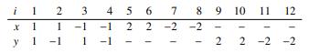
with missing observations marked as “–”.
Let y denote the observed data. Let z = {x9, . . . , x12, y5, . . . , y8} denote the missing data. Find p(z | Σ, µ, y) and h(µ, Σ | y,z).
Hint: Write h(µ, Σ | y,z) as h(Σ | y,z) · h(µ | Σ, y,z).

c. Data augmentation – algorithm. Using the conditional posterior distributions found in part (b), describe a data augmentation scheme to implement posterior simulation from h(µ, Σ | y).
• Set up a Gibbs sampler for h(µ, Σ,z | y). Let θ
k = (µ
k , Σ
k ,z k ) denote the simulated Monte Carlo sample, k = 1, . . . , K.
• Simply drop the z k . The remaining (µ
k , Σ
k ) are an MC sample from h(µ, Σ | y).

d. Data augmentation – simulation. Implement the data augmentation described in part (c). Plot trajectories of generated µj , j = 1, 2, against iteration number and estimated marginal posterior distributions h(µj | y).

e. Convergence diagnostic. Propose some (ad hoc) convergence diagnostic to decide when to terminate posterior simulation in the program used for part (d).

(The answer need not be perfect – any reasonable, practical, creative suggestions is fine. See Section 9.6 for more discussion of convergence diagnostics.)

(xi, yi) N(u,E), i = 1,....n.