7–96 Solving Differential Equations with MATLAB MATLAB has a built-in function for solving ordinary differential equations called dsolve. We can use this function to quickly explore the solution to a second-order differential equation when the forcing function is a sinusoidal or exponential signal.

Suppose we have a series RLC circuit in the zero state connected to a voltage source vTðtÞ. The parameter values are R=4 kΩ, L= 1 H, and C= 1 μF. The differential equation for the voltage across the capacitor is given by Eq. (7–33). If vTðtÞ = 10 uðtÞ V, we can use the following MATLAB code to solve for the capacitor voltage and plot the results.

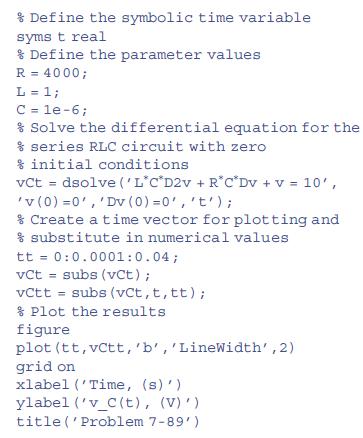
Run the given MATLAB code and examine the results. Modify the code to solve the same problem when the input voltage is vTðtÞ = 10 cosð200 πtÞ V. Solve the problem a third time for vTðtÞ = 10e−2000t V. Compare and comment on the responses for the three different types of input signals.

Define the symbolic time variable syms t real Define the parameter values R = 4000; L = 1; C = le-6; * Solve the differential equation for the series RLC circuit with zero % initial conditions vCtdsolve ('L'C'D2v + R*C*Dv + v = 10', 'v (0)=0', 'Dv (0)=0', 't'); * Create a time vector for plotting and substitute in numerical values tt 0:0.0001:0.04; vCt subs (vCt); vCtt subs (vCt, t, tt); % Plot the results figure plot (tt, vctt, 'b', 'LineWidth', 2) grid on xlabel('Time, (s)') ylabel ('v_C(t), (V)') title('Problem 7-89')