Develop a script to generate the same computations and plots as in Sec. 21.8, but for the MATLAB peaks function over ranges of both x and y from –3 to 3.

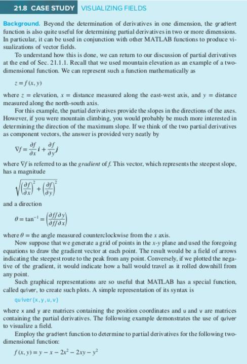
21.8 CASE STUDY VISUALIZING FIELDS Background. Beyond the determination of derivatives in one dimension, the gradient function is also quite useful for determining partial derivatives in two or more dimensions. In particular, it can be used in conjunction with other MATLAB functions to produce vi- sualizations of vector fields. To understand how this is done, we can return to our discussion of partial derivatives at the end of Sec. 21.1.1. Recall that we used mountain elevation as an example of a two- dimensional function. We can represent such a function mathematically as z=f(x,y) where z = elevation, x = distance measured along the east-west axis, and y = distance measured along the north-south axis. For this example, the partial derivatives provide the slopes in the directions of the axes. However, if you were mountain climbing, you would probably be much more interested in determining the direction of the maximum slope. If we think of the two partial derivatives as component vectors, the answer is provided very neatly by of Vf=i+ where Vf is referred to as the gradient of f. This vector, which represents the steepest slope. has a magnitude and a direction 0=tan where 0 = the angle measured counterclockwise from the x axis. Now suppose that we generate a grid of points in the x-y plane and used the foregoing equations to draw the gradient vector at each point. The result would be a field of arrows indicating the steepest route to the peak from any point. Conversely, if we plotted the nega- tive of the gradient, it would indicate how a ball would travel as it rolled downhill from any point. Such graphical representations are so useful that MATLAB has a special function, called quiver, to create such plots. A simple representation of its syntax is quiver (x, y,u,v) where x and y are matrices containing the position coordinates and u and v are matrices containing the partial derivatives. The following example demonstrates the use of quiver to visualize a field. Employ the gradient function to determine to partial derivatives for the following two- dimensional function: f(x,y)=y-x-21-2xy-y