Repeat the the same simulations as in Section 22.6 for the Lorenz equations but generate the solutions with the midpoint method.

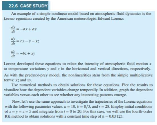
22.6 CASE STUDY An example of a simple nonlinear model based on atmospheric fluid dynamics is the Lorenz equations created by the American meteorologist Edward Lorenz: =-ox+y =rx-y-xz =-bz + xy Lorenz developed these equations to relate the intensity of atmospheric fluid motion x to temperature variations y and z in the horizontal and vertical directions, respectively. As with the predator-prey model, the nonlinearities stem from the simple multiplicative terms: xz and xy. Use numerical methods to obtain solutions for these equations. Plot the results to visualize how the dependent variables change temporally. In addition, graph the dependent variables versus each other to see whether any interesting patterns emerge. Now, let's use the same approach to investigate the trajectories of the Lorenz equations with the following parameter values: a = 10,b=8/3, and r= 28. Employ initial conditions of x=y=z=5 and integrate from t=0 to 20. For this case, we will use the fourth-order RK method to obtain solutions with a constant time step of h = 0.03125.