Figure P2.21a shows a uniform beam subject to a linearly increasing distributed load. As depicted in Fig. P2.21b, deflection y (m) can be computed with

where E = the modulus of elasticity and I = the moment of inertia (m⁴). Employ this equation and calculus to generate MATLAB plots of the following quantities versus distance along the beam:
(a) Displacement (y),
(b) Slope [θ(x) = dy/dx],
(c) Moment [M(x) = EId² y/dx²],
(d) Shear [V(x) = EId³ y/dx³], and
(e) Loading [w(x) = −EId⁴ y/dx⁴].
Use the following parameters for your computation:
L = 600 cm, E = 50,000 kN/cm², I = 30,000 cm⁴, w₀ = 2.5 kN/cm, and Δx = 10 cm. Employ the subplot function to display all the plots vertically on the same page in the order (a) to (e). Include labels and use consistent MKS units when developing the plots.

Figure P2.21b:

Transcribed Image Text:

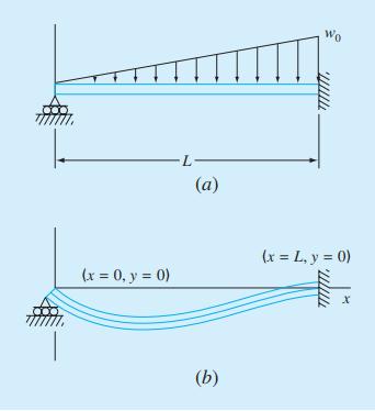
y = wo 120EIL -(-x² + 2L²x³ - L²x)