How would you change the MDP representation of Section 13.3 to a POMDP? Take the simple robot

Question:

How would you change the MDP representation of Section 13.3 to a POMDP? Take the simple robot problem and its Markov transition matrix created in Section 13.3.3 and change it into a POMDP. Think of using a probability matrix for the partially observable states.

Data from section 13.3

In Section 10.7 we first introduced reinforcement learning, where with reward reinforcement, an agent learns to take different sets of actions in an environment. The goal of the agent is to maximize its long-term reward. Generally speaking, the agent wants to learn a policy, or a mapping between reward states of the world and its own actions in the world.

To illustrate the concepts of reinforcement learning, we consider the example of a recycling robot (adapted from Sutton and Barto 1998). Consider a mobile robot whose job is to collect empty soda cans from business offices. The robot has a rechargeable battery. It is equipped with sensors to find cans as well as with an arm to collect them. We assume that the robot has a control system for interpreting sensory information, for navigating, and for moving its arm to collect the cans. The robot uses reinforcement learning, based on the current charge level of its battery, to search for cans. The agent must make one of three decisions:

1. The robot can actively search for a soda can during a certain time interval;

2. The robot can pause and wait for someone to bring it a can; or 3. The robot can return to the home base to recharge its batteries.

The robot makes decisions either in some fixed time period, or when an empty can is found, or when some other event occurs. Consequently, the robot has three actions while its state is being determined by the charge level of the battery. The reward is set to zero most of the time, it becomes positive once a can is collected, and the reward is negative if the the battery runs out of energy. Note that in this example the reinforcement-based learning agent is a part of the robot that monitors both the physical state of the robot as well as the situation (state) of its external environment: the robot-agent monitors both the state of the robot as well as its external environment.

There is a major limitation of the traditional reinforcement learning framework that we have just described: it is deterministic in nature. In order to overcome this limitation and to be able to use reinforcement learning in a wider range of complex tasks, we extend the deterministic framework with a stochastic component. In the following sections we consider two examples of stochastic reinforcement learning: the Markov decision process and the partially observable Markov decision process.

Data from section 13.3.3

To illustrate a simple MDP, we take up again the example of the recycling robot (adapted from Sutton and Barto 1998) introduced at the beginning of Section 13.3. Recall that each time this reinforcement learning agent encounters an external event it makes a decision to either actively search for a soda can for recycling, we call this search, wait for someone to bring it a can, we call this wait, or return to the home base to recharge its battery, recharge. These decisions are made by the robot based only on the state of the energy level of the battery. For simplicity, two battery levels are distinguished, low and high: the state space of S = {low, high}. If the current state of the battery is high, the battery is charged, otherwise it’s state is low. Therefore the action sets of the agent are A(low) = {search, wait, recharge} and A(high) = {search, wait}. If A(high) included recharge, we would expect the agent to learn that a policy using that action would be suboptimal!

The state of the battery is determined independent of actions taken. If it is high, then we expect that the robot will be able to complete a period of active search without the risk of running down the battery. Thus, if the state is high, then the agent stays in that state with probability a and changes its state to low with probability 1-a. $3If the agent decides to perform an active search while being in state low, the energy level of the battery remains the same with probability b and the battery runs out of energy with probability 1- b.

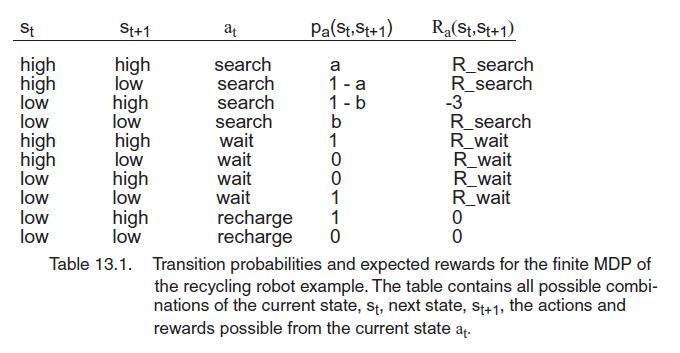
We next create a reward system: once the battery is run down, S = low, the robot is rescued, its battery is recharged to high, and it gets a reward of -3. Each time the robot finds a soda can, it receives a reward of 1. We denote the expected amount of cans the robot will collect (the expected reward the agent will receive) while actively searching and while it is waiting by Research and R wait and assume that R_search > R_wait. We also assume that the robot cannot collect any soda cans while returning for recharging and that it cannot collect any cans during a step in which the battery is low. The system just described may be represented by a finite MDP whose transition probabilities (pa (st, st+1)) and expected rewards are given in Table 13.1.

To represent the dynamics of this finite MDP we can use a graph, such as Figure 13.13, the transition graph of the MDP for the recycling robot. A transition graph has two types of nodes: state nodes and action nodes. Each state of the agent is represented by a state node depicted as a large circle with the state's name, s, inside. Each state-action pair is represented by an action node connected to the state node denoted as a small black circle.

If the agent starts in state s and takes action a, it moves along the line from state node s to action node (st , a). Consequently, the environment responds with a transition to the next state's node via one of the arrows leaving action node (st, a), where each arrow corresponds to a triple (st, a, st+1), where st+1 is the next state. The arrow is labeled with the

St high high low low high high low low low low St+1 high low high low high low high low high low Table 13.1.

transition probability, p_a(s_t, s_t+1), and the expected reward for the transition, R_a(s_t , s_t+1), is represented by the arrow. Note that the transition probabilities associated with the arrows leaving an action node always sum to 1. We see several of the stochastic learning techniques described in this chapter again in Chapter 15, Understanding Natural Language.