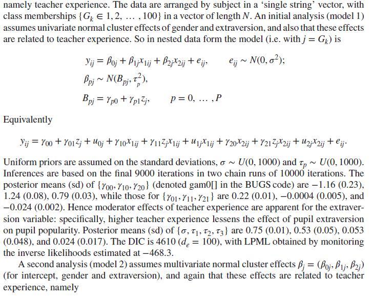
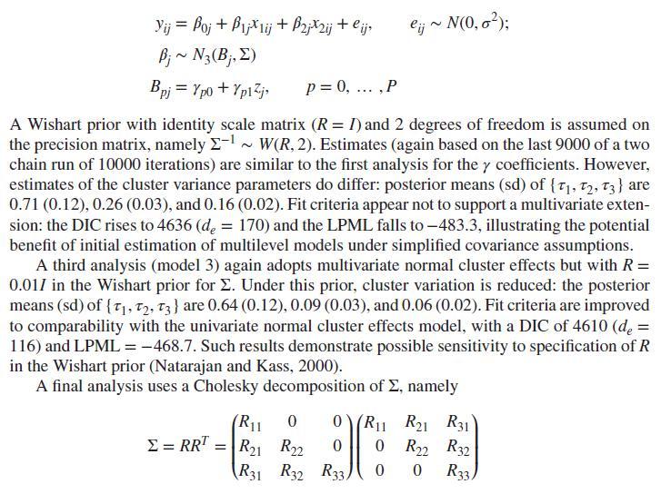
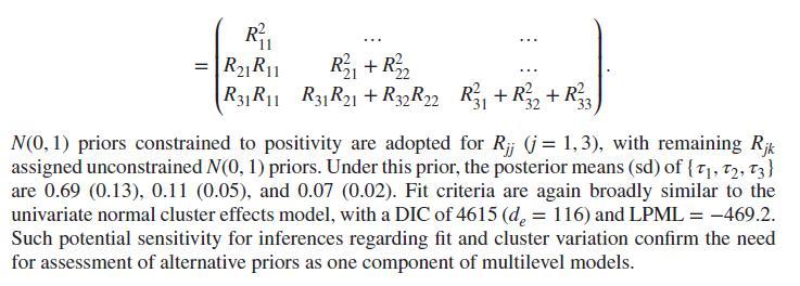
In Example 5.6, and assuming a Wishart prior \((R=0.01 I\) as the scale matrix \()\) on the second stage precision matrix (model 3), assess the assumption of level 1 homoscedasticity. It is suggested to monitor \(\mu_{i j}\), and realised values of the standardised level 1 residuals \(e_{i j}^{s}=\left(y_{i j}-\mu_{i j}\right) / \sigma\), and obtain their posterior means. One can then see whether the residual variance changes according to grouped categories of \(\mu_{i j}\) (e.g. deciles). Alternatively one may plot posterior mean \(e_{i j}^{s}\), or their squares, against the posterior means of \(\mu_{i j}\) or against the predictors. One may also estimate linear regressions of the squares of the posterior mean \(e_{i j}^{s}\) against polynomial functions of the posterior mean \(\mu_{i j}\). Analysis of this kind suggests a quadratic relation between the error variance and the posterior mean \(\mu_{i j}\).

Data from Example 5.6

Transcribed Image Text:

Consider two level continuous data, namely pupil popularity scores y;; for N = 2000 pupils in J = 100 school classes (the clusters). At level 1 there are P = 2 predictors, gender xiij (1=girl, 0=boy), and a measure of extraversion X2ij. At level 2 there is a single predictor Zj,