Methods And Applications Of Linear Models Regression And The Analysis Of Variance 2nd Edition Ronald R. Hocking - Solutions

Develop the matrices to express the hypotheses in (12.2), (12.4) and (12.6) in the form H-0.
An experiment was conducted to determine the weight gains of laboratory animal under nine feeding regimes in a completely randomized design. The treatments were defined as all combinations of factor A. three sources of protein, beef, pork, and grain, and factor B, three amounts of protein, low,
Suppose you have the following incidence matrix, and assume the two- factor model 011 10 11 101a. Determine the A-effect hypotheses corresponding to (11.69), (11.70), and (11.72).b. Determine the effective interaction hypothesis.c. Assuming the no-interaction model, determine the effective model
In Exercise 10.14 we discussed a comparison of fluids used to combat the buildup of lactic acid. Those data can be modeled as a two-factor experiment with factor one, with two levels, being the type of drink, A or B. Since the drinks are prepared by adding a powder to water, we can consider adding
Verify the hypotheses implied by the two computing methods in Example 11.7,
For the missing cell problem of Exercise 11.24, consider the model where we have set y = 0,1 and 2, 0, otherwise.a. Using any scheme to remove the degeneracy in the design matrix, show that the estimates of the design parameters are correct.b. Show that the estimate of 6 is , as defined in Exercise
Consider the two-factor, no-interaction model with one observation per cell except that = 0 for the case a 2 and 6-3.a. Show that the estimate of p, is given by ay. + by y.. (a-1)(b-1)b. It is suggested that the missing observation be replaced by and the data analyzed as if it was the actual
For the incidence matrices in Example 11.2, use the matrix reduction method implied in (11.98) to show that for the no-interaction model all parameters are estimable for (a) and (b) but not for (c). Show that the design matrix for the first two cases have full column rank.
Consider the no-interaction model in (11.73) with cell means estimates given by (11.75). Show that the sample cell means, are unbiased for p this model but have greater variance than
Suppose we use the parameterization in (11.45). hypotheses associated with the sums of squares defined by R(ap. B. (a) and R((a), 8). Section 11.3
Verify that the sequential method tests the hypotheses H** Determine the
a. In the proportional frequencies model from Example 11.4, show that the hypotheses Hand HA++ are identical.b. Write the parameter matrix corresponding to the conditions in (11.71) and describe the new parameters in terms of the cell means.c. Write the normal equations in terms of these parameters
a. Verify the degeneracy in the design matrix for Example 11.3.1b. Write the normal equations after setting (a) = 0, and determine the solution.c. Verify that the apparent estimate of p, follows from the constraint imposed on the cell means.
Write normal equations for the marginal-means reparameterized, unconstrained, unbalanced two-factor model, noting the lack of orthogonality. Note that the solution is given by substituting the cell means estimates into the defining relations in (11.38).
Suppose the main effect hypothesis is given by the relations in (11.45). Determine the effective hypotheses based on these hypotheses for the three incidence matrices in Example 11.2. Section 11.2.2
Describe the estimate of 2 in (11.65) if some cell have n = 0. Note the associated degrees of freedom.
a. Verify the estimate of 8 in (11.57). Hint: Recall the development of the analysis of covariance described in Exercise 10.15.b. Verify the expression for Ng in (11.58).c. Verify the expression for Nin (11.63).
Box, Hunter, and Hunter (1978) describe a two-factor experiment in which all combinations of three poisons (factor A) and four antidotes (factor B) are considered. Four replicates (laboratory animals) are randomly allocated to each treatment combination. The survival times are shown in the
Suppose that we remove the redundancies in the over-parameterized model by imposing the conditions ox. == 0 and (a) = (a) = 0 for all / and j. Show that this leads to the same test statistics as if we had used the parameter matrix P defined in (11.43).
Use the parameter matrix in (11.43) to transform to a full rank set of equations. Note the structure of the coefficient matrix. Verify that the solution of this set of equations is given by substituting the cell means estimates into (11.45).
a. Use (11.42) to write the normal equations for the over-parameterized, two- way classification model.b. Show that sweeping on the diagonal elements in the natural order corresponds using the parameter matrix in (11.43).e. Use the parameter matrix defined in (11.36) to transform the normal
Show that the numerator sum of squares for testing the hypothesis H,, defined in (11.29), is given by (11.30). Do this algebraically and in matrix form by writing the appropriate hypothesis matrix and applying the general result. Section 11.1.4
a. For Example 11.1 use the Scheff half-width to test the significance of the interaction contrasts that are suggested by Figure 11.1a. Contrast this with the conclusions using the separate-r method.b. Apply the expression for the most significant linear function from Chapter 18 to identify the
Show that the sums of squares for the main effects hypotheses and the interaction hypotheses add to the sum of squares for the hypothesis of equal means. This provides an illustration of Cochran's theorem, described in Chapter 16. Use both the algebraic and the Kronecker product expressions for the
Verify the expression for the constrained estimator in (11.23). Hint: Use the Lagrange multiplier approach. Give an intuitive argument for the result.
Use the expression for the expected value of the non-central x distribution to verify the relation between the non-centrality parameter and the expected mean square in (11.21).
a. Verify the matrix expressions for the hypotheses, HAB, and HA, in (11.17).b. Verify (11.18) and the relations in (11.19).
For the two-factor model, develop the expression for the main effect hypothesis, HB, test statistic for this hypothesis, the expected mean square and the associated constrained estimator.
Verify the expression for the constrained estimator in (11.13). Hint: Use the LaGrange multiplier approach. Give an intuitive argument for the result.
a. Verify the Kronecker product expression for the residual sum of squares in (11.3).b. Verify the Kronecker product expression for N, in (11.4), either by using the algebraic expression or by writing the hypothesis in matrix form and applying the general expression in (10.14).
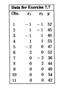
An experiment was conducted to measure the effect of four drugs on the response y to a particular stimulus. Since the individuals in the study may not be identical in their response to the drugs, their response z to the stimulus prior to taking the drug was measured. The data are shown in the
For the model in (10.72):a. Write the normal equations for and .b. Solve the equations for as a function of , use this result to eliminate j from the equation and solve for . Use this result to solve for p.c. Verify the expression for Ny.d. Verify the expression for N.
Hocking (1985) describes an experiment for comparing five fluids that are supposed to prevent the buildup of lactic acid in long-distance runners. For reasons unrelated to the fluids, there were an unequal number of runners assigned to the treatments. The sample means, sample variances, and cell
a. For the unbalanced, one-way classification model, write the design matrix WX,P for each of the two transformed models defined by (10.52) and (10.54) for the case p = 4.b. Develop the transformation matrix for the parameterization suggested by (10.61). That is, define a " and a,,-, for i=1,..,
For the balanced, cell means model, with p = 5, develop the numerator sum of squares for testing the hypothesis H = and 44 = Ms. Section 10.3
Ostle and Malone (1988) describe an experiment conducted to examine five different electrolytes used in batteries. The data are given in the following table: Data for Exercise 10.11 Electrolyte Obs. 1 2 3 4 5 1 40 38 44 41 34 2 45 40 42 43 35 31 46 38 40 40 34 4 49 44 34 40 33a. Assuming the usual
a. Assuming that the balanced, one-way classification model is written in over- parameterized form as in (10.55), write the normal equations and observe that the coefficient matrix is singular. Using the methods for determining generalized inverses, described in Appendix A.1.12, determine a
The first form of the hypothesis in (10.7) is not of the form (10.50) and hence the relation given in (10.47) and (10.48) does not hold. However, it is reasonable to consider the transformation in (10.46) using H, as defined in (1.8). Determine the expression for j in terms ofa. Hint: To determine
a. Verify the relation in (10.48) as follows: Solve the relation as eu for j use (10.47) to write the relation in terms of a,, and then note that J=0.b. Use the expression for a in terms of a to write Mb. Use the fact that MMI to show that, under the restriction imposed by the requirement in
a. Verify that the columns of A in (10.44) are eigenvectors of HHT and determine the associated eigenvalues.b. Let and denote the last two columns of A and verify that +vy and y are also eigenvectors and contrasts that are orthogonal to v, but not to each other.
Develop the matrix expression for the numerator sum of squares Ny in (10.20) by using HA, as defined in (10.9).
Write the design matrix, X = WX,P for the parameterization in (10.52)
a. Verify the expression in Equation (10.41) for the contrast sum of squares.b. Verify the relation in (10.42). Hint: Let A be the matrix whose columns are the eigenvectors,a, and show that the sums of squares for the hypotheses, H: Hp Oand H ATH 0 are identical. Then use the properties of the
The source of the significant F-ratio may not be revealed by either the simultaneous acceptance intervals or the projection ellipses. It is shown in Chapter 18 that the most significant single degree-of-freedom hypothesis has the form H: a H-0, where =(H(WW)'H)'Hp.a. Using the results form the
a. Verify the results in Equations (10.17) and (10.18).b. Show that the expression in Equation (10.19) agrees with the expression for Ny in Equation (10.12).c. Verify the expression for Ny in (10.22).
Assuming the balanced cell means model in Equation (10.1):a. Show that WTW nl,, WWT 1, U., and WTy = Col[y].b. Show that I - W(ww)w = 1, S..c. Verify that Equations (10.3) and (10.4) give the same expression for RSS.d. Show that the rank of S,, is (n - 1).
In the two sample problem described in Example 9.2, write the covariance matrix if it is assumed that the two populations have different variances, and
Let =(\) be an arbitrary covariance matrix of size three. Write Vin the form
Suppose all variances are equal, Varly, and all covariances are equal, Cory Determine the matrices V and V to write the covariance matrix in the form V=V+V
For the two-factor, mixed model described in Example 9.4, write out the covariance matrix associated with the structure described algebraically in (9.20), and in matrix form in (9.21), for the case a = 3, b-2
Consider an experiment designed to compare the response to two different fertilizers, each at three different amounts. The two-factor cell means model is appropriate with ; denoting the mean response of the jth amount of the ith fertilizer. Suppose that the lowest level of each fertilizer is zero.
Consider the no-interaction, two-factor model with a 2 and b = 3.a. Show that a non-redundant set of constraints is given by for j=1,2.b. Use these relations to replace 1 and 2 and write the reduced model in algebraic form.c. Write the design matrix for this reduced model.
Consider the two-factor model in Equation (9.15) with a 6-2. Write the design matrix associated with the reparameterization given by 01411421 841-12 12 11 12 1433 +1422- Comment on the implications of testing the hypotheses, H: 012 =0, HA: 0 0 and Hp : 02 0.
a. Suppose A and B are matrices of dimensions (axa) and (b, x b). What is the dimension of A & B?b. Write out explicit expressions for the Kronecker products, IJ, JOI, UI. IU,UJ and JU, where I and U are 3 x 3 and J is 2 x 1. 9.4 For the model in Equation (9.14), describe how you would use
Use the regression methodology to develop estimates of andand to develop an algebraic expression for the test statistic for the hypothesis, H 14=14
Use the regression methodology to develop the estimates for and in Example 9.1 and also to develop an algebraic expression for the test statistic for the hypothesis, Hoo
Assume that (y, z) follow an (m + 1)-variate normal distribution with mean vector (.) and covariance matrix V = y Vaa. From the conditional distribution of y given z, described in Chapter 16, show that the conditional moments are where = Vy E[x] =+ (x-4) Varly] yb. Suppose z is partitioned into ar,
Verify the expression for the expected value of 1/x2(v) and the expression for the unconditional variance of B, in (8.53).
Generate data for the model E[y] and try fitting a two-variable quadratic model. Contrast your result with that obtained by Friedman and Stuetzle (1981) to illustrate the projection pursuit method. Section 8.4
If computer software is available, use any of the non-parametric methods in Section 8.2 to fit the Indianapolis 500 data (Appendix D, Table D.4) and compare the result with that from Exercise 7.22. Section 8.3
If computer software is available, use any of the non-parametric methods in Section 8.2 to fit the highway fatality data (Appendix D, Table D.3) for the years 1950-1974 and compare the result with that from Exercise 7.21.c.
Verify the expression for the gradient vector in (8.23) and the derivative in (8.24) to establish the fact that Q(t) is decreasing in the Gauss-Newton direction. Section 8.2
Alternative methods for minimizing Q(0) are based on either first-order or second-order steepest descent. These are defined as: first-order: g(+1) 816, where 6 is the negative of the gradient vector to Q(0) evaluated at " second order: g+)-1H-18, where H is the matrix of second derivatives
a. Spell out the details of the Gauss-Newton computations for the modelb. Using the following data, perform one iteration with initial values = 580, 180, and 0=-0.16. 0 Data for Exercises 8.2 and 8.3 127 151 379 421 460 426 -5-3 -13 5
a. Use a non-linear regression program to fit the Forbes data in Table 2.2 to the Clausius-Clapeyson equation PR=TexP(459.7+ BP)b. Compare the parameter estimates and variance estimates with those obtained using the linearization in Chapter 3.c. Specify different initial values for the parameters
IQ scores of identical twins, one raised in a foster home (y) and the other raised by natural parents (2) are categorized by three social classes of the natural parents. The objective is to examine the relation between the scores of the twins as a function of social class. The following indicator
In Exercise 2.10 we examined the data shown in Appendix D, Table D.4. that shows winning speeds at the Indianapolis 500 for the years 1911 - 1971, excluding the war years 1917-1918 and 1942-1945. It is conjectured that technology changes during the wars may have introduced discontinuities into the
In Exercise 2.9 we discussed the data in Appendix D, Table D.3, that relates highway fatalities (FATAL) and number of licensed vehicles (NOV) for the years 1950-1979, fitting a linear and a quadratic model. Noting that the speed limit was reduced from 65 to 55 mph in the last five years of this
In Exercise 4.7, we discussed the data in Appendix D, Table D.7, that relate gas mileage (MPG) to certain characteristics of the automobile. Here we focus on displacement (DISP) and type of transmission, where we define the indicator { 1 if automatic 0 if manual.a. Fit the model MPG=+B,DISP+e,
Write the model for fitting quadratic segments for power demand as in Figure 7.10. Applications
a. Use the growth data from Table 7.8 to fit quadratic segments for Age < 7 and Age 7 and plot the fitted equations.b. Refit the data forcing continuity at Age 7 and plot the fitted equations.c. Refit the data forcing a smooth fit and plot the fitted equations.
Write a model for fitting linear segments to power demand as indicated in Figure 7.10.
a. Write the equations for the two cases, Age
Fit a quadratic equation to the growth data in Table 7.9 and examine the residual plots for an indication that the segmented model should be used.
In Example 7.8, we suggested two different schemes for coding the qualitative variables.a. Suppose you had fit four separate equations for the four groups with coefficients (0,0), (7). (b) and (PP). Relate these coefficients to the 8, and B, in (7.31) and (7.33).b. A third alternative coding for
Referring to Example 7.4, define Gen 1 for males and Gen-1 for females, and define the interaction term as usual..a. Relate the coefficients in this form of the model to the coefficients in the separate models.b. Write the normal equations for fitting this model.
Verify algebraically the assertion made in Example 7.6 that the i-statistic for the coefficient of the indicator variable is identical to the r-statistic for the comparison of means.
Starting with the design matrix written as in (7.14) with vectors J, J. x, and x and parameter vector , rewrite the model in terms of the parameter vector and design matrix 21 J z= J 2 Ja. Describe the relation between the parameter vectors.b. Determine the matrix M which relates X and Z, or
Using the data from Example 7.4, test (a), the hypotheses of equal slopes (b), the hypothesis of equal intercepts and (c) the hypothesis of identical lines using the model in the form of (7.18).
Determine the transformation matrix M that relates X and Z in (7.14) and (7.18). Use this matrix to verify the parameter relations in (7.19).7.9 Using the data from Example 7.4:a. Fit the model in the form of (7.14) and again in the form of (7.17) and use the difference in residual sum of squares
The data in the following table were collected to examine a response surface:a. Fit a second-order model to the data, and compute the stationary point.b. Determine the eigenvalues of B, and describe the surface.c. Use the method of ridge analysis to describe the optimum response and its location as
Lawson (1979) examined the flowability (F) of a coal slurry as a function of two additives. The data are shown in the following table (a= 1.15, b = 3.29, c=2.21). The experiment initially considered three factors, each at two levels, with some replication. The third factor was eliminated,
Richburg (1989) describes the use of extrusion in the production of snack foods. In a study of the properties of one process, she examined the bulk density (D) of the product as a function of the moisture of the feed (M) at three levels (-1.25,0, 1.25) and the screw speed (R) at three levels
Using the fitted equation from Exercise 7.1:a. Determine the stationary point of the fitted surface.b. Determine the eigenvalues of the matrix of second-order coefficients, and note that the stationary point is neither a maximizer nor a minimizer.e. Use the method of ridge analysis to determine the
Verify the solution, given in (7.10), for the constrained optimization problem in (7.9).
a. Using the data in Table 7.1, fit the twisted plane model in (7.6).b. Plot the contours in the (Time, Temp)-plane for fixed values of strength, and contrast with Figure 7.1.c. Plot the contours in the (STR-Temp)-plane for fixed values of Time, and contrast with Figure 7.2. Section 7.2
Myers (1976) discusses an experiment to study the yield (MBT) of a chemical process as a function of Time and Temperature. The fitted equation in terms of scaled variables is MBT -82.17-1.01 Time -8.61 Temp + 1.40Time -8.76Temp -7.20(Time Temp) Plot the contours (Time Temp), (MBT-Time) and (MBT
In Appendix D, Table D.14, we show data taken from Brownlee (1960) showing a response and three predictors. These data were used to illustrate the concept of variable selection. (See also Draper and Smith (1981).) The data were also used by Andrews (1974) to illustrate the robust methods discussed
Analyze the steel data, Appendix D, Table D.5 for unusual observations. Determine the case diagnostics, added-variable and principal component plots, and compare the latter with the scatter-plots from Exercise 4.4. Recall the consequences of deleting case 3 on the collinearity indicatoes as
a. Develop a computer program to implement the Huber robust algorithm as defined by equation (6.57)b. Write a computer program to implement the function in equation (6.58).e. Use these methods to analyze the dilemma data for N = 26 and N = 27, and comment on the effectiveness of the methods with
Fit the dilemma data with N-27 observations, and verify the case diagnostics is Table 6.4. Prepare the added-variable, principal component and augmented principal component plots and examine them for evidence of unusual observations.
Show that the augmented, centered Hat matrix may be written as in equation (6.47) with diagonal elements given in equation (6.48). Hin: Use the partitioned form to obtain (44))
Develop the expression for the projection ellipse in equation (6.43). Hint: Consider a tangent plane, at a", to the ellipsoid (2-2) M(-)-1 defined by the vector a (a,ay, 0, 0), and consider the first two elements of this vector. The locus of all such points then defines the projection ellipse
Determine the prediction equation for the dilemma data using orthogonal regression, as described in Exercise 5.8, and compare with the least squares fit. Section 6.6
Extensions of the analysis of the dilemma data. Refit the data with case 24 deleted, but with case 17 retained to see if this case is still outlying.b. Determine the collinearity in Example 6.1 with cases 17 and 24 deleted. Use both the eigenvector and the regression among predictors and compare
Show that r, and RSS, are independent. (Hint: Lets be the unit vector defined in Exercise 6.7 and show that rw-y. Use this relation to write RSS as a quadratic form on y and use the result on the independence of linear and quadratic forms given in Theorem 16.6.) Section 6.5
Suppose that case i is an outlier, in the sense that an amount & is added to its expected value. Let be the unit vector with one in the ith position and zeros elsewhere and write the revised model is y=XB++. Weisberg (1985) calls this the mean shift outlier model. Using standard methodology,
Belsley, Kuh, and Welsch (1980) proposed the statistics DFBETAS, to assess the effect of the ath case on the estimate of 8. Here var='s Show that if we use var,-al in the denominator this statistic is identical to the Studentized residual.
In equation (6.39), the difference - was scaled by an estimate of the variance of to obtain the statistic, DFFITS, Show that if we scale by the estimated variance in equation (6.41), the statistic is identical to the Studencized residual.
Verify the result given in equation (6.32).

Showing 400 - 500 of 1264

Methods And Applications Of Linear Models Regression And The Analysis Of Variance 2nd Edition Ronald R. Hocking - Solutions

Step by Step Answers