New Semester Started Get 50% OFF Study Help! --h --m --s Claim Now

Question Answers

Textbooks

Find textbooks, questions and answers

Oops, something went wrong!

Change your search query and then try again

Result Not Found

Books FREE
Study Help
Tutors
AI Study Planner NEW
Sell Books

Search
Sign In
Register

study help
business
microeconomics principles applications

Microeconomic Theory Basic Principles And Extensions 1st Edition Christopher M Snyder, Walter Nicholson, Robert B Stewart - Solutions

What are the budget constraints in these two alternative scenarios? How is income distributed between wages and profits in each case? Explain the differences intuitively.
How would an increase in the total amount of labour available shift the production possibility frontiers in these examples?
11.9 Cobweb models One way to generate disequilibrium prices in a simple model of supply and demand is to incorporate a lag into producer’s supply response. To examine this possibility, assume that quantity demanded in period t depends on price in that period (Q D t = a − bPt )but that quantity
11.8 The Ramsey formula for optimal taxation The development of optimal tax policy has been a major topic in public finance for centuries.17 Probably the most famous result in the theory of optimal taxation is due to the English economist Frank Ramsey, who conceptualised the problem as how to
11.7 Ad valorem taxes Given an ad valorem tax rate of t, the gap between the price consumers pay and what suppliers receive is given by PD = (1 + t)PS.a. Show that for an ad valorem tax d In PD dt=eS eS − eD and d In Ps dt=eD es − eD.b. Show that the excess burden of a small tax is DW = −0.5
11.6 Suppose that the market demand for a product is given by QD = A – BP. Suppose also that the typical firm’s cost function is given by C(q) = k + aq + bq2.a. Compute the long-run equilibrium output and price for the typical irm in this market.b. Calculate the equilibrium number of irms in
11.5 The domestic demand for MP3 players is given by Q = 5000 − 100P, where price (P) is measured in Euros and quantity (Q)is measured in thousands of MP3 players per year. The domestic supply curve for MP3 players is given by Q = 150P.a. What is the domestic equilibrium in the MP3 players
11.4 The swimming pool maintenance sector consists of 100 identical firms, each having short-run total costs given by STC = 0.5q 2 + 10q + 5 and short-run marginal costs given by SMC = q + 10, where q is the number of swimming pools serviced per day.a. What is the short-run supply curve for each
11.3 Suppose that the demand for skateboard is given by Q = 1500 − 50P and that the long-run total operating costs of each skateboard manufacturer in a competitive industry are given by C(q) = 0.5q 2 − 10q.Entrepreneurial talent for skateboard manufacturing is scarce. The supply curve for
11.2 Assume each firm in a perfectly competitive market has an identical cost structure such that long-run average cost is minimised at an output of 20 units (qi = 20). The minimum average cost is €10 per unit. Total market demand is given by Q = 1500 − 50P.a. What is the industry’s long-run
11.1 Suppose there are 50 identical firms in a perfectly competitive industry. Each firm has a short-run total cost function of the form TC = 0.2q 2 + 5q + 10.a. Calculate the irm’s short-run supply curve with q as a function of market price (P).b. On the assumption that there are no interaction
Can you explain intuitively why the marginal burden of a tax exceeds its average burden? Under what conditions would the marginal excess burden of a tax exceed additional tax revenues collected?
How does the size of the total welfare loss from a quantity restriction depend on the elasticities of supply and demand? What determines how the loss will be shared?
How do the total, marginal and average functions derived from Equation 11.55 differ from those in Example 11.4? Are costs always greater (for all levels of q) for the former cost curve? Why is long-run equilibrium price higher with the former curves? (See footnote 10 for a formal discussion.)
Presumably, the entry of frame makers in the long run is motivated by the short-run profitability of the industry in response to the increase in demand. Suppose each firm’s short-run costs were given SC = 50q 2 − 1500q + 20 000.Show that short-run profits are zero when the industry is in
Do the results of changing auto workers’ wages agree with what might have been predicted using an equation similar to Equation 11.30?
How would the results of this example change by assuming different values for the weight of labour in the production function (i.e., for α and β)?
For this linear case, when would it be possible to express market demand as a linear function of total income (I1 + I2)? Alternatively, suppose the individuals had differing coefficients for py . Would that change the analysis in any fundamental way?
10.9 Le Châtelier’s Principle Because firms have greater flexibility in the long run, their reactions to price changes may be greater in the long run than in the short run. Paul Samuelson was perhaps the first economist to recognise that such reactions were analogous to a principle from physical
10.8 Some envelope results Young’s theorem can be used in combination with the envelope results to derive some useful results.a. Show that ∂l (P, v, w) /∂v = ∂k (P, v, w) /∂w using substitution and output effects.b. Use the result from part (a) to show how a unit tax on labour would be
10.7 How would you expect an increase in output price, P, to affect the demand for capital and labour inputs?a. Explain graphically why, if neither input is inferior, it seems clear that a rise in P must not reduce the demand for either factor.b. Show that the graphical presumption from part (a)is
10.6 This problem concerns the relationship between demand and marginal revenue curves for a few functional forms.a. Show that, for a linear demand curve, the marginal revenue curve bisects the distance between the vertical axis and the demand curve for any price.b. Show that, for any linear demand
10.5 Would a lump-sum profits tax affect the profit- maximising quantity of output? How about a proportional tax on profits? How about a tax assessed on each unit of output?How about a tax on labour input?
10.4 QuickLearn Driving School trains learner drivers.The number of candidate drivers it can train per week is given by q = 10 min(k, l )′, where k is the number of vehicles the firm hires per week, l is the number of instructors hired each week, and g is a parameter indicating the returns to
10.3 The production function for a firm in the business of calculator assembly is given by q = 2!l, where q denotes finished calculator output and l denotes hours of labour input. The firm is a price-taker both for calculators (which sell for P) and for workers (which can be hired at a wage rate of
10.2 Universal Widget produces high-quality widgets at its plant in Johannesburg, South Africa for sale throughout the world.The cost function for total widget production (q) is given by TC = 0.1q 2 + 100.Widgets are demanded only in Austria (where the demand curve is given by qA = 50 − 2PA) and
10.1 Harry’s Hardware is a small business that sells bags of cement in a market where it is a price-taker and P = MR The prevailing market price of cement is €10 per 50 kg bag. Harry’s total cost function is given by TC = 0.05q 2 + 5q + 22 where q is the number of bags of cement Harry chooses
How would the calculations in this problem be affected if all firms had experienced the rise in wages?Would the decline in labour (and capital) demand be greater or smaller than found here?
How is the amount of short-run producer surplus here affected by changes in the rental rate for capital, v?How is it affected by changes in the wage, w?
How would you graph the short-run supply curve in Equation 10.22? How would the curve be shifted if w rose to 15? How would it be shifted if capital input increased to k1 = 100? How would the short-run supply curve be shifted if v fell to 2? Would any of these changes alter the firm’s
Suppose demand depended on other factors in addition to p . How would this change the analysis of this example? How would a change in one of these other factors shift the demand curve and its marginal revenue curve?
How would an increase in the marginal cost of sandwich production to €5 affect the output decision of this firm? How would it affect the firm’s profits?
9.12 Suppose the total-cost function for a firm is given by C = qw 2 /3V 1/3.a. Use Shephard’s lemma to compute the (constant output) demand functions for inputs l and k.b. Use your results from part (a) to calculate the production function for q.
9.11 A firm producing polo sticks has a production function given by q = 2!kl .In the short run, the firm’s amount of capital equipment is fixed at k = 100. The rental rate for k is v = £1 and the wage rate for l is w = £4.a. Calculate the irm’s short-run total cost curve.Calculate the
9.10 Suppose that a firm’s fixed proportion production function is given by q = min(5k, 10l ).a. Calculate the irm’s long-run total, average and marginal cost functions.b. Suppose that k is ixed at 10 in the short run.Calculate the irm’s short-run total, average, and marginal cost
9.9 Suppose that a firm produces two different outputs, the quantities of which are represented by q1 and q2. In general, the firm’s total costs can be represented by C(q1, q2).This function exhibits economies of scope if C(q1, 0) +C(0, q2) > C(q1, q2) for all output levels of either good.a.
9.8 Show that Euler’s theorem implies that, for a constant returns-to-scale production function [q = f (k, l )], q = fk · k + fl · l .Use this result to show that, for such a production function, if MPl > APl then MPk must be negative. What does this imply about where production must take
9.7 Consider a generalisation of the production function in Example 9.3:q = β0 + β1!kl + β2k + β3l , where 0 ≤ βi ≤ 1, i = 0,…, 3.a. If this function is to exhibit constant returns to scale, what restrictions should be placed on the parameters β0, … , β3?b. Show that, in the constant
9.6 Suppose we are given the constant returns-to-scale CES production function q = [k ρ + l ρ]1/ρ.a. Show that MPk = (q/k)1–ρ and MPl = (q/l)1–ρ.b. Show that RTS = (k /l)1–ρ; use this to show thatσ = 1/(1 – ρ).c. Determine the output elasticities for k and l; and show that their sum
9.5 The general Cobb–Douglas production function for two inputs is given by q = f (k, l ) = AkαIβ, where 0 < α < 1 and 0 < β < 1. For this production function:a. Show that fk > 0, f1 > 0, fkk < 0, fll < 0, and fkl =flk > 0.b. Show that eq, k = α and eq, l = β.c. Scale elasticity can be
9.4 Suppose that the quantity of plastic bottles produced (q)takes place in two locations. Capital inputs cannot change and changes in production use only labour as an input. The production function in location 1 is given by q1 = 10l 0.5 1and in the other location by q2 = 50l 0.5 2 .a. If a single
9.3 Basil Fawlty is planning to renovate the restaurant in his hotel.The production function for new restaurant tables is given by q = 0:1k 0:2l 0:8, where q is the number of restaurant tables produced during the renovation week, k represents the number of hours of table manufacturing machines used
9.2 Suppose the production function for product x is given by q = kl − 0.8k 2 − 0.2l 2,where q represents the annual quantity of product x produced, k represents annual capital input and l represents annual labour input.a. If k = 10, graph the total and average productivity of labour curves. At
9.1 TransFast Trucking Company uses two sizes of trailers for transportation contracts. Smaller trailers can carry 2 tons and larger trailers can carry 4 tons.a. TransFast Trucking Company is awarded a contract to cart 8000 kilograms of cargo. Construct an isoquant for the irst production function.
Explain why an increase in w will increase both short-run average cost and short-run marginal cost in this illustration, but an increase in v affects only short-run average cost.
How would total costs change if w increased from 12 to 27 and the production function took the simple linear form q = k + 4l ? What light does this result shed on the other cases in this example?
In this example, what are the elasticities of total costs with respect to changes in input costs? Is the size of these elasticities affected by technical change?
How are the various substitution possibilities inherent in the CES function reflected in the CES cost function in Equation 9.96?
In the Cobb–Douglas numerical example with w/v = 4, we found that the cost minimising input ratio for producing 40 units of output was k /l = 80/20 = 4. How would this value change for σ = 2 or σ = 0.5? What actual input combinations would be used? What would total costs be? Total cost function
Actual studies of production using the Cobb–Douglas tend to find α ≈ 0.3. Use this finding together with Equation 9.67 to discuss the relative importance of improving capital and labour quality to the overall rate of technical progress.
What can you learn about this production function by graphing the q = 4 isoquant? Why does this function generalise the fixed-proportions case?
For cases where k = l, what can be said about the marginal productivities of this production function?How would this simplify the numerator for Equation 9.21? How does this permit you to more easily evaluate this expression for some larger values of k and l ?
qUERY: How would an increase in k from 10 to 11 affect the MPl and APl functions here? Explain your results intuitively.
8.12 refinements of perfect Bayesian equilibrium Recall the job-market signalling game in Example 8.9.a. Find the conditions under which there is a pooling equilibrium where both types of worker choose not to obtain an education (NE) and where the irm offers an uneducated worker a job. Be sure to
8.11 Alternatives to Grim strategy Suppose that the Prisoners’ Dilemma stage game (see Figure 8.1) is repeated for infinitely many periods.a. Can players support the cooperative outcome by using tit-for-tat strategies, punishing deviation in a past period by reverting to the stage-game Nash
8.10 rotten Kid theorem In A Treatise on the Family (Cambridge, MA: Harvard University Press, 1981), Nobel laureate Gary Becker proposes his famous Rotten Kid Theorem as a sequential game between the potentially rotten child (player 1) and the child’s parent (player 2). The child moves first,
8.9 fairness in the Ultimatum Game Consider a simple version of the Ultimatum Game discussed in the text. The first mover proposes a division of €1. Let r be the share received by the other player in this proposal (so the first mover keeps 1 – r), where 0 ≤ r ≤ 1/2. Then the other player
8.8 In Blind Poker, player 2 draws a card from a standard deck and places it against her forehead without looking at it but so player 1 can see it. Player 1 moves first, deciding whether to stay or fold. If player 1 folds, he must pay player 2 €50. If player 1 stays, the action goes to player 2.
8.7 Return to the game with two security guards in Problem 8.4. Continue to suppose that player i’s average benefit per hour of work on landscaping is 10 − li +lj 2.Continue to suppose that guard 2’s opportunity cost of an hour of perimeter patrolling work is 4. Suppose that guard 1’s
8.6 The following game is a version of the Prisoners’ Dilemma, but the payoffs are slightly different than in Figure 8.1.2a. Verify that the Nash equilibrium is the usual one for the Prisoners’ Dilemma and that both players have dominant strategies.b. Suppose the stage game is repeated
8.5 The Academy Award–winning movie A Beautiful Mind about the life of John Nash dramatises Nash’s scholarly contribution in a single scene: his equilibrium concept dawns on him while in a bar bantering with his fellow male graduate students. They notice several women, one blond and the rest
8.4 Two security guards employed by different companies, i = 1, 2, simultaneously choose how many hours li to spend patrolling a street. The average benefit per hour can be expressed as 10 − li +lj 2and the (opportunity) cost per hour for each is 4.Security guard i’s average benefit is
8.3 The game of Chicken is played by two macho teens who speed toward each other on a single-lane road. The first to veer off is branded the chicken, whereas the one who does not veer gains peer-group esteem. Of course, if neither veers, both die in the resulting crash. Payoffs to the Chicken game
8.2 The mixed-strategy Nash equilibrium in the Battle of the Sexes in Figure 8.3 may depend on the numerical values for the payoffs. To generalise this solution, assume that the payoff matrix for the game is given bywhere K ≥ 1. Show how the mixed-strategy Nash equilibrium depends on the value of
8.1 Consider the following game:a. Find the pure-strategy Nash equilibria (if any).b. Find the mixed-strategy Nash equilibrium in which each player randomises over just the irst two actions.c. Compute players’ expected payoffs in the equilibria found in parts (a) and (b).d. Draw the extensive
To complete our analysis: In this equilibrium, type H of player 1 cannot prefer to deviate from E. Is this true? If so, can you show it? How does the probability of type L trying to ‘pool’ with the high type by obtaining an education vary with player 2’s prior belief that player 1 is the high
Return to the pooling outcome in which both types of player 1 obtain an education. Consider player 2’s posterior beliefs following the unexpected event that a worker shows up with no education. Perfect Bayesian equilibrium leaves us free to assume anything we want about these posterior beliefs.
Suppose herder 1 is the high type. How does the number of sheep each herder grazes change as the game moves from incomplete to full information (moving from point C ′ to C )? What if herder 1 is the low type? Which type prefers full information and thus would like to signal its type? Which type
If the probability that player 1 is of type t = 6 is high enough, can the first candidate be a Bayesian–Nash equilibrium? If so, compute the threshold probability.
How would the Nash equilibrium shift if both herders’ benefits increased by the same amount? What about a decrease in (only) herder 2’s benefit from grazing?
What is a player’s expected payoff in the Nash equilibrium in strictly mixed strategies? How does this payoff compare with those in the pure-strategy Nash equilibria? What arguments might be offered that one or another of the three Nash equilibria might be the best prediction in this game?
What is the husband’s expected payoff in each case? Show that his expected payoff is 2 – 2h – 2w + 3hw in the general case. Given the husband plays the mixed strategy (4/5, 1/5), what strategy provides the wife with the highest payoff?
QUerY: Does any player have a dominant strategy? Why is (paper, scissors) not a Nash equilibrium?
7.14 the portfolio problem with a normally distributed risky asset In Example 7.3 we showed that a person with a CARA utility function who faces a Normally distributed risk will have expected utility of the form E [U (W )] = μW − (A/2)σ2 W ′where μW is the expected value of wealth and σ2 W
7.13 Graphing risky investments Investment in risky assets can be examined in the state-preference framework by assuming that W * Euros invested in an asset with a certain return r will yield W *(1 + r) in both states of the world, whereas investment in a risky asset will yield W *(1 + rg) in good
7.12 More on the CrrA function For the CRRA utility function (Equation 7.42), we showed that the degree of risk aversion is measured by 1 – R. In Chapter 3 we showed that the elasticity of substitution for the same function is given by 1/(1 – R). Hence the measures are reciprocals of each
7.11 Prospect theory Two pioneers of the field of behavioural economics, Daniel Kahneman and Amos Tversky (winners of the Nobel Prize in economics in 2002), conducted an experiment in which they presented different groups of subjects with one of the following two scenarios:● Scenario 1: In
7.10 HArA Utility The CARA and CRRA utility functions are both members of a more general class of utility functions called harmonic absolute risk aversion (HARA) functions. The general form for this function is U(W ) = θ (μ + W/γ)1−γ, where the various parameters obey the following
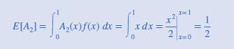
7.9 Return to Example 7.5, in which we computed the value of the real option provided by a flexible-fuel car. Continue to assume that the payoff from a fossil-fuel-burning car is A1(x) = 1 − x. Now assume that the payoff from the biofuel car is higher, A2(x) = 2x. As before, x is a random
7.8 In Equation 7.30 we showed that the amount an individual is willing to pay to avoid a fair gamble (h) is given by p = 0.5E (h 2)r (W ), where r (W ) is the measure of absolute risk aversion at this person’s initial level of wealth. In this problem we look at the size of this payment as a
7.7 A farmer believes there is a 50–50 chance that the next growing season will be abnormally rainy. His expected utility function has the form expected utility =1 2ln YNR +1 2ln YR , where YNR and YR represent the farmer’s income in the states of ‘normal rain’ and ‘rainy’,
7.6 In deciding to sell a counterfeited product illegally, an individual knows that the probability of getting caught by the police is p and that the fine the individual will have to pay if apprehended isf. Suppose that all individuals are risk averse(i.e., U ″(W ) < 0, where W is the
7.5 A three-month safari to the Okavango Delta in Botswana is estimated to cost Amy €10 000. The utility from the safari is a function of how much she actually spends on it (Y), given by U (Y ) = ln Y.a. If there is a 25 per cent probability that Amy will lose €1000 of her cash on the safari,
7.4 A health insurance company considers the risk to a Sherpa who has a current wealth of 20 000 renminbi (RMB), working in the Himalayas, incurring an injury in the performance of their duties which that will cost 10 000 RMB in medical care is 50 per cent.a. Calculate the cost of actuarially fair
7.3 An individual purchases a dozen eggs and must take them home. Although making trips home is costless, there is a 50 per cent chance that all the eggs carried on any one trip will be broken during the trip. The individual considers two strategies: (1) take all 12 eggs in one trip; or (2) take
7.2 Show that if an individual’s utility-of-wealth function is convex then he or she will prefer fair gambles to income certainty and may even be willing to accept somewhat unfair gambles. Do you believe this sort of risk-taking behaviour is common? What factors might tend to limit its occurrence?
7.1 George is seen to place an even-money £100 000 bet on Manchester United to win the English Premier League Final. If George has a logarithmic utility-of-wealth function and if his current wealth is £1 000 000, what must he believe is the minimum probability that the Manchester United will win?
Does risk aversion always increase option value? If so, explain why. If not, modify the example with different shapes to the payoff functions to provide an example where the risk neutral buyer would pay more. Let’s work out the option value provided by a flexible-fuel car in a numerical example.
With the constant relative risk aversion function, how does this person’s willingness to pay to avoid a given absolute gamble (say, of 1000) depend on his or her initial wealth?
Suppose this person had two ways to invest his or her wealth: Allocation 1, μ1 = 107 000 and σ1 = 10 000;Allocation 2, μ2 = 102 000 and σ2 = 2000. How would this person’s attitude toward risk affect his or her choice between these allocations?15
Suppose utility had been linear in wealth. Would this person be willing to pay anything more than the actuarially fair amount for insurance? How about the case where utility is a convex function of wealth?
Here are two alternative solutions to the St Petersburg paradox. For each, calculate the expected value of the original game.1. Suppose individuals assume that any probability less than 0.01 is in fact zero.2. Suppose that the utility from the St Petersburg prizes is given by if x 1 000 000, U(x)=
6.8 separable utility A utility function is called separable if it can be written as U (x, y) = U1(x) + U2(y), where U ′i > 0, U i″ < 0, and U1, U2 need not be the same function.a. What does reparability assume about the crosspartial derivative Uxy? Give an intuitive discussion of what word
6.7 Consumer surplus with many goods The welfare costs of changes in a single price can be measured using expenditure functions and compensated demand curves. This problem asks you to generalise this to price changes in two (or many) goods.a. Suppose that an individual consumes n goods and that the
6.6 Example 6.3 computes the demand functions implied by the three-good CES utility function U (x, y, z) = −1 x−1 y−1 z.a. Use the demand function for x in Equation 6.32 to determine whether x and y or x and z are gross substitutes or gross complements.b. How would you determine whether x and
6.5 In general, uncompensated cross-price effects are not equal. That is,�xi�pj≠�xj�pi Use the Slutsky equation to show that these effects are equal if the individual spends a constant fraction of income on each good regardless of relative prices.(This is a generalisation of Problem 6.1.)
6.4 A pensioner allocates her budget between three commodities, bread (b), tuna (t) and prune juice (p). If the ratio of the price of tuna to bread is a constant pt pb:a. How might one deine a composite commodity for the pensioner’s solid food consumption?b. State the pensioner’s optimisation
6.3 A migrant farm worker consumes only two goods, coffee(c) and buttered toast (bt) that he obtains from the local take-away. Buttered toast is a composite commodity consisting of a single slice of toast and two grams of butter.The migrant worker chooses to allocate his budget equally between
6.2 Monica is currently unemployed and consumes two goods to sustain her, chicken giblets and rice. Monica considers chicken giblets an inferior good that exhibits Giffen’s paradox, although chicken giblets and rice are Hicksian substitutes in the customary sense. Develop an intuitive explanation
6.1 Johannes Jacobus (JJ) receives utility from two goods, mampoer (liquor) (m) and steak (s)U (m, s) = m · s.a. Prove that an increase in the price of mampoer will not inluence JJ’s consumption of steak.b. Show also that ∂m/∂ps = 0.c. Use the Slutsky equation and the symmetry of net

Showing 3300 - 3400 of 6303

First
27
28
29
30
31
32
33
34
35
36
37
38
39
40
41
Last

Step by Step Answers

Services

Sitemap
Fun
Definitions
Become Tutor
Used Textbooks
Study Help Categories
Recent Questions
Expert Questions
Campus Wear
Sell Your Books

Company Info

Security
Copyrights
Privacy Policy
Terms & Conditions
SolutionInn Fee
Scholarship
Online Quiz
Give Feedback, Get Rewards

Get In Touch

About Us
Contact Us
Career
Jobs
FAQ
Student Discount
Campus Ambassador

Secure Payment

Download Our App

© 2026 SolutionInn. All Rights Reserved