New Semester
Started
Get
50% OFF
Study Help!
--h --m --s
Claim Now
Question Answers
Textbooks
Find textbooks, questions and answers
Oops, something went wrong!
Change your search query and then try again
S
Books
FREE
Study Help
Expert Questions
Accounting
General Management
Mathematics
Finance
Organizational Behaviour
Law
Physics
Operating System
Management Leadership
Sociology
Programming
Marketing
Database
Computer Network
Economics
Textbooks Solutions
Accounting
Managerial Accounting
Management Leadership
Cost Accounting
Statistics
Business Law
Corporate Finance
Finance
Economics
Auditing
Tutors
Online Tutors
Find a Tutor
Hire a Tutor
Become a Tutor
AI Tutor
AI Study Planner
NEW
Sell Books
Search
Search
Sign In
Register
study help
business
model based testing for embedded systems
Introduction To Robust Estimation And Hypothesis Testing 3rd Edition Rand R. Wilcox - Solutions
Repeat Exercise 6, only now use the rank-based method in Section 8.6.12.
Analyze the data in Table 6.1 using the methods in Sections 8.6.1 and 8.6.4.
Repeat Exercises 3 and 4 using the data for the murderers in Table 6.1.
Repeat Exercise 3 using the rank-based method in Section 8.5. How do the results compare to using a measure of location?
Analyze the data for the control group reported in Table 6.1 using the methods in Sections 8.1 and 8.2. Compare and contrast the results.
For the data used in Exercise 1, compute confidence intervals for all pairs of trimmed means using the R function pairdepb.
Section 8.6.2 reports data on hangover symptoms. For group 2, use the R function rmanova to compare the trimmed means corresponding to times 1, 2, and 3.
For the schizophrenia data in Section 7.8.4, compare the groups with t1way and pbadepth.
Generate data for a 2-by-3 design and use the function pbad2way. Note the contrast coefficients for interactions. If you again use pbad2way, but with conall=F, what will happen to these contrast coefficients? Describe the relative merits of using conall=T.
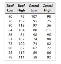
Snedecor and Cochran (1967) report weight gains for rats randomly assigned to one of four diets that varied in the amount and source of protein. The results were as follows:Verify the results based on the R function pba2way mentioned in the example of Section 7.7.1. Beef Beef Cereal Cereal Low High
For the data in the previous two exercises, perform all pairwise comparisons using the Harrell–Davis estimate of the median.
For the data in the previous exercise, compare the groups using both the Rust–Fligner and Brunner–Dette–Munk methods.
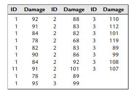
Suppose three different drugs are being considered for treating some disorder, and it is desired to check for side effects related to liver damage. Further suppose that the following data are collected on 28 participants.The values under the columns headed by ID indicate which of the three drugs a
Using the data from the previous two exercises, compare the 20% trimmed means of the experimental group to the control taking into account grade. Also test for no interactions using lincon and linconb. Is there reason to suspect that the confidence interval returned by linconb will be longer than
Using the data in the previous exercise, use the function lincon to compare the experimental group with the control group taking into account grade and the two tracking abilities. (Again, tracking abilities 2 and 3 are combined.) Comment on whether the results support the conclusion that the
Some psychologists have suggested that teachers’ expectancies influence intellectual functioning. The file VIQ.dat contains pretest verbal IQ scores for students in grades 1 and 2 who were assigned to one of three ability tracks. (The data are from Elashoff and Snow, 1970, and originally
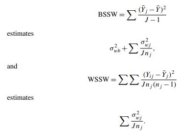
From well-known results on the random effects model (e.g., Graybill, 1976;Jeyaratnam and Othman, 1985), it follows that Use these result to derive an alternative estimate of ρWI. estimates BSSW= (-Y) J-1 + Jnj and WSSW= (Yij-;) Jn (n; - 1) estimates Jnj
If data are generated from exponential distributions, what problems would you expect in terms of probability coverage when computing confidence intervals? What problems with power might arise?
Describe how M-measures of location might be compared in a two-way design with a percentile bootstrap method. What practical problem might arise when using the bootstrap and sample sizes are small?
For the data in Table 6.6, compare the groups using the method in Section 6.8.
Argue that when testing Eq. (6.27), this provides a metric-free method for comparing groups based on scatter.
For the data in Table 6.1, compare the two groups with the method in Section 6.12.
For the data in Table 6.1, compare the two groups with the method in Section 6.11.
For the data in Table 6.1, compare the two groups with the method in Section 6.10.
For the data in Table 6.1, compare the two groups with the method in Section 6.8.
For the cork boring data in Table 6.5, imagine that the goal is to compare the north, east and south sides to the west side How might this be done with the software in Section 6.6.1? Perform the analysis and comment on the results. (The data are stored in the file corkall.dat; see Chapter 1.)
The file read.dat contains data from a reading study conducted by L. Doi. Columns 4 and 5 contain measures of digit naming speed and letter naming speed. Use both the relplot and the MVE method to identify any outliers. Compare the results and comment on any discrepancies.
The MVE method of detecting outliers, described in Section 6.4.3, could be modified by replacing the MVE estimator of location with the Winsorized mean, and replacing the covariances with the Winsorized covariances described in Section 5.9.3. Discuss how this would be done and its relative merits.
The average LSAT scores (X) for the 1973 entering classes of 15 American law schools, and the corresponding grade point averages (Y ), are as follows.Use a boxplot to determine whether any of the X values are outliers. Do the same for the Y values. Comment on whether this is convincing evidence
Give a general description of a situation where for n = 20, the minimum depth among all points is 3/20.
Suppose that for each row of an n-by-p matrix, its depth is computed relative to all n points in the matrix. What are the possible values that the depths might be?
Repeat the last two exercises, but now use the data in Table 6.2.
Repeat the last exercise using the data for group 2.
For the data in Table 6.1, check for outliers among the first group using the methods in Section 6.4. Comment on why the number of outliers found differs among the methods.
Repeat the last exercise using the data for group 2.
For the EEG data in Table 6.1, compute the MVE, MCD, OP, and the Donoho–Gasko.2 trimmed mean for group 1.
Using R, generate 30 observations from a standard normal distribution and store the values in x. Generate 20 observations from a chi-squared distribution with one degree of freedom and store them in z. Compute y=4(z-1), so x and y contain data sampled from distributions having identical means.
Let D = X −Y , let θD be the population median associated with D, and let θX and θY be the population medians associated with X and Y , respectively. Verify that under general conditions, θD 6= θX −θY .
The file tumor.dat contains data on the number of days to occurrence of a mammary tumor in 48 rats injected with a carcinogen and subsequently randomized to receive either the treatment or the control. The data were collected by Gail, Santner, and Brown(1980) and represent only a portion of the
Continuing the last exercise, examine a boxplot of the data. What would you expect to happen if the 0.95 confidence interval is computed using a bootstrap-t method? Verify your answer using the R function yuenbt.
The file pyge.dat (see Section 1.8) contains pretest reasoning IQ scores for students in grades 1 and 2 who were assigned to one of three ability tracks. (The data are from Elashoff & Snow, 1970, and originally collected by R. Rosenthal.) The file pygc.dat contain data for a control group. The
Section 5.9.6 used some hypothetical data to illustrate the R function yuend with 20%trimming. Use the function to compare the means. Verify that the estimated standard error of the difference between the sample means is smaller than the standard error of the difference between the 20% trimmed
The example at the end of Section 5.3.3 examined some data from an experiment on the effects of drinking alcohol. Another portion of the study consisted of measuring the effects of alcohol over 3 days of drinking. The scores for the control group, for the first 2 days of drinking, are 4, 47, 35, 4,
Compute a confidence interval for p using the data in Table 5.1.
Comment on the relative merits of testing H0: p = 1/2 with Mee’s method versus comparing two independent groups with the Kolmogorov–Smirnov test.
Describe a situation where testing H0: p = 1/2 with Mee’s method can have lower power than the Yuen–Welch procedure.
Apply the Yuen–Welch method to the data in Table 5.1 where the amount of trimming is 0, 0.05, 0.1, and 0.2. Compare the estimated standard errors of the difference between the trimmed means.
Verify that if X and Y are independent, the third moment about the mean of X −Y isµx[3] −µy[3].
Compare the deciles only, using the Harrell–Davis estimator, using the data in Table 5.1.
Consider two independent groups having identical distributions. Suppose four observations are randomly sampled from the first and three from the second. Determine P(D = 1) and P(D = 0.75), where D is given by Eq. (5.4). Verify your results with the R function kssig.
Summarize the relative merits of using the weighted versus unweighted Kolmogorov–Smirnov test. Also discuss the merits of the Kolmogorov–Smirnov test relative to comparing measures of location.
Compare the two groups of data in Table 5.3 using the weighted Kolmogorov–Smirnov test. Plot the shift function and its 0.95 confidence band. Compare the results with the unweighted test.
Compare the two groups of data in Table 5.1 using the weighted Kolmogorov–Smirnov test. Plot the shift function and its 0.95 confidence band. Compare the results with the unweighted test.
Generate 20 observations from a g-and-h distribution with g = h = 0.5. (This can be done with the R function ghdist, written for this book.) Examine a boxplot of the data.Repeat this 10 times. Comment on the strategy of examining a boxplot to determine whether the confidence interval for the mean
For the LSAT data in Table 4.3, compute a 0.95 bootstrap-t confidence interval for mean using the R function trimcibt with plotit=T. Note that a boxplot finds no outliers.Comment on the plot created by trimcibt in terms of achieving accurate probability coverage when using Student’s t. What does
Verify Eq. (4.5) using the decision rule about whether to reject H0 described in Section 4.4.3.
Discuss the relative merits of using the R function sint versus qmjci and hdci.
For the exponential distribution, would the sample median be expected to have a relatively high or low standard error? Compare your answer to the estimated standard error obtained with data generated from the exponential distribution.
Do the skewness and kurtosis of the exponential distribution suggest that the bootstrap-t method will provide a more accurate confidence interval for µt versus the confidence interval given by Eq. (4.3)?
If the exponential distribution has variance µ[2] = σ2, then µ[3] = 2σ3 and µ[4] = 9σ4.Determine the skewness and kurtosis. What does this suggest about getting an accurate confidence interval for the mean?
The R function rexp generates data from an exponential distribution. Use R to estimate the probability of getting at least one outlier, based on a boxplot, when sampling from this distribution. Discuss the implications for computing a confidence interval for µ.
Use the R functions qmjci, hdci, and sint to compute a 0.95 confidence interval for the median based on the LSAT data in Table 4.3. Comment on how these confidence interval compare to one another.
Compute a 0.95 confidence interval for the mean, 10% mean, and 20% mean using the lifetime data listed in the example of Section 4.6.3. Use both Eq. (4.3) and the bootstrap-t method.
Compute a 0.95 confidence interval for the mean, 10% mean, and 20% mean using the data in Table 3.1 of Chapter 3. Examine a boxplot of the data and comment on the accuracy of the confidence interval for the mean. Use both Eq. (4.3) and the bootstrap-t method
Describe situations where the confidence interval for the mean might be too long or too short. Contrast this with confidence intervals for the 20% trimmed mean and µm.
Verify that Eq. (3.29) reduces to s 2/n if no observations are flagged as being unusually large or small by 9.
Argue that if 9 is taken to be the biweight, it approximates the optimal choice for 9 under normality when observations are not too extreme.
Set Xi = i, i = 1, . . . , 20 and compute the Harrell–Davis estimate of the median. Repeat this, but with X20 equal to 1000 and then 100,000. When X20 = 100,000, would you expect xˆ0.5 or the Harrell–Davis estimator to have the smaller standard error? Verify your answer.
Repeat the previous exercise, only this time compute the biweight midvariance, the 20%Winsorized variance, and the percentage bend midvariance. Comment on the resistance of these three measures of scale.
Next, set X20 = 200 and compute both estimates of location. Replace X19 with 200 and again estimate the measures of location. Keep doing this until the upper half of the data is equal to 200. Comment on the resistance of the M-estimator versus 20% trimming.
Use results on Winsorized expected values in Chapter 2 to show that X¯ w is a Winsorized unbiased estimate of µw. 9. Set Xi = i, i = 1, . . . , 20, and compute the 20% trimmed mean and the M-estimate of location based on Huber’s
Use results on Winsorized expected values in Chapter 2 to show that if the error term in Eq. (3.4) is ignored, X¯t is a Winsorized unbiased estimate of µt.
Cushny and Peebles (1904) conducted a study on the effects of optical isomers of hyoscyamine hydrobromide in producing sleep. For one of the drugs, the additional hours of sleep for 10 patients were 0.7, −1.6, −0.2, −1.2, −0.1, 3.4, 3.7, .8, 0, and 2.Compute the Harrell–Davis estimate of
Comment on the strategy of applying the boxplot to the data in Exercise 2, removing any outliers, computing the sample mean for the data that remain, and then estimating the standard error of this sample mean based on the sample variance of the data that remain.
For the data in Exercise 1, estimate the deciles using the Harrell–Davis estimator. Do the same for the data in Table 3.2. Plot the difference between the deciles as a function of the estimated deciles for the data in Exercise 1. What do the results suggest? Estimate the standard errors
For the data in Exercise 1, compute MADN, the biweight midvariance, and the percentage bend midvariance. Compare the results to those obtained for the data in Table 3.2. What do the results suggest about which group is more dispersed?
In the study by Dana (1990) on self-awareness, described in this chapter (in connection with Table 3.2), a second group of subjects yielded the observations 59 106 174 207 219 237 313 365 458 497 515 529 557 615 625 645 973 1065 3215.Compute the sample median, the Harrell–Davis estimate of the
Included among the R functions written for this book is the function ghdist(n,g=0,h=0)which generates n observations from a so-called g-and-h distribution (which is described in more detail in Chapter 4). The command ghdist(30,0,.5) will generate 30 observations from a symmetric, heavy-tailed
Showing 4600 - 4700
of 4678
First
33
34
35
36
37
38
39
40
41
42
43
44
45
46
47
Step by Step Answers