The following data are from an experiment that tested the performance of an industrial engine (Schlotzhauer and Littell 1997). The experiment used a mixture of diesel fuel and gas from distilling organic materials.

Write and execute a SAS program to perform the computations to provide answers to the following questions. Extract material from the output and copy or attach them as the required answers.

a. Use the method of least squares to obtain estimates βˆ0 and βˆ1 of the parameters in the model y = β0 + β1x + .

b. Construct a plot that shows the scatter of (x, y) data points with y on the vertical axis.

c. Give the least squares prediction equation. Superimpose the least squares line on the scatter plot in part (b).

d. Compute a table of predicted values ˆy and residuals y−yˆ corresponding to the observed values y.

e. Identify the sums of squares (y−y¯)2, (ˆy−y¯)2, and (y−yˆ)2 from your output. Verify that these give a decomposition of total variability in y into two parts and identify the parts by sources of variation.

f. Calculate the proportion of the total variability in the y-values that is accounted for by the linear regression model. Explain why this value is a measure of how well your model fits the data.
g. Give the point estimate s2 of σ2.
h. State the estimated standard errors of βˆ0 and βˆ1.
i. Construct 95% confidence intervals for β0 and β1.
j. Test the hypothesis H0 : β1 = 0 versus Ha : β1 = 0 using a t-test.
Give your conclusion using α = 0.05 and the p-value.

k. Obtain plots of the residuals against x and the predicted values, respectively. Do these two plots suggest any inadequacies of this model?

Explain why you reached your conclusion.

l. Obtain a normal probability plot of the studentized residuals. State the model assumption that you can verify using this plot. Is this a plausible assumption for this model?

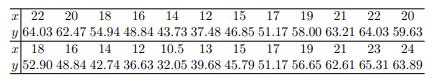
x 22 20 18 16 14 12 15 17 19 21 22 20 y 64.03 62.47 54.94 48.84 43.73 37.48 46.85 51.17 58.00 63.21 64.03 59.63 218 16 14 12 10.5 13 15 17 19 21 23 24 y 52.90 48.84 42.74 36.63 32.05 39.68 45.79 51.17 56.65 62.61 65.31 63.89