

Question: Derive the transfer function for the LTI model in Examples 10-3 and 10-4 using weighted least squares. Manipulate the weights and test whether the transfer
Derive the transfer function for the LTI model in Examples 10-3 and 10-4 using weighted least squares.
Manipulate the weights and test whether the transfer function can be identified with lesser number of measurements used in the examples. You may use a maximum tolerance of 10-3 for the estimation error between the identified transfer function coefficients and their actual values.
Example 10-3
Suppose that a first-order system yields the following data: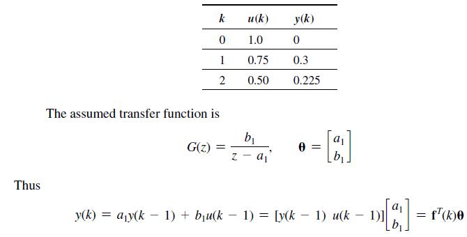
![[] 0 = y(k)= ay(k 1) + bu(k - 1) = [y(k-1)](https://dsd5zvtm8ll6.cloudfront.net/images/question_images/1705/6/4/4/07065aa102641e691705644069265.jpg)
Example 10-4
Consider the input and output data of a LTI system with sampling time T = 0.1 s:![u(k DI[a] = f'(k)0](https://dsd5zvtm8ll6.cloudfront.net/images/question_images/1705/6/4/4/08965aa10396aa3c1705644088397.jpg)
We wish to generate the least-squares estimate of the transfer function from the given input–output data. For this one may write a simple MATLAB code using the function arx as follows.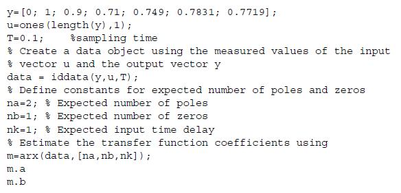
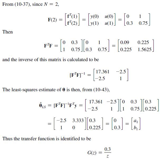
Thus k 0 1 2 The assumed transfer function is G(z) = u(k) 1.0 0.75 0.50 b z a y(k) 0 0.3 0.225 - [] 0 = y(k)= ay(k 1) + bu(k - 1) = [y(k-1) u(k DI[a] = f'(k)0
Step by Step Solution
3.44 Rating (160 Votes )
There are 3 Steps involved in it

Get step-by-step solutions from verified subject matter experts