Write a MATLAB program to perform a simulation of the solution of Exercise 1.22.

(i) Simulate the continuous-time signals \(x_{\mathrm{a}}(t)\) in MATLAB using sequences obtained by sampling them at 100 times the sampling frequency, that is, as \(f_{\mathrm{s}}(m)=\) \(f_{\mathrm{a}}(m(T / 100))\). The sampling process to generate the discrete-time signal is then equivalent to keeping 1 out of 100 samples of the original sequence, forming the signal \(f(n)=f_{\mathrm{s}}(100 n)=f_{\mathrm{a}}(n T)\).
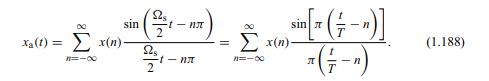
(ii) The interpolation in Equation (1.188) can be approximated by truncating each function \[\frac{\sin \left[\pi\left(\frac{t}{T}-n\right)\right]}{\pi\left(\frac{t}{T}-n\right)}\]
considering them to be zero outside the time interval \(n T-10 T \leq t \leq n T+10 T\). Note that, since we are truncating the interpolation functions, the summation in Equation (1.188) needs to be carried out only for a few terms.

 Exercise 1.22.

Suppose we want to process the continuous-time signal

\[x_{\mathrm{a}}(t)=3 \cos (2 \pi 1000 t)+7 \sin (2 \pi 1100 t)\]

using a discrete-time system. The sampling frequency used is 4000 samples per second. The discrete-time processing carried out on the signal samples \(x(n)\) is described by the following difference equation.

\[y(n)=x(n)+x(n-2) .\]

After the processing, the samples of the output \(y(n)\) are converted back to continuoustime form using Equation (1.188). Give a closed-form expression for the processed continuous-time signal \(y_{\mathrm{a}}(t)\). Interpret the effect this processing has on the input signal.

Transcribed Image Text:

Xa(t) = x(n)- 11=18 sin 2 - 1 = x(n)- 11=-00 sin [(+-)] JT n (1.188)