Residential Demand for Electricity. Belotti, Hughes and Piano Mortari (2017) estimated residential demand for electricity covering the

Question:

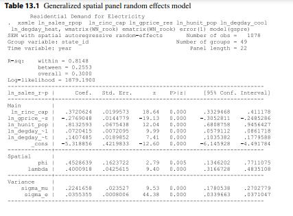
Residential Demand for Electricity. Belotti, Hughes and Piano Mortari (2017) estimated residential demand for electricity covering the 48 states in the continental United States plus the district of Columbia for the period 1990-2010.

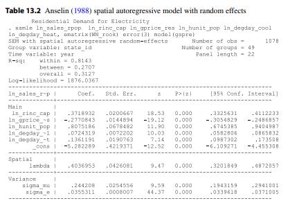
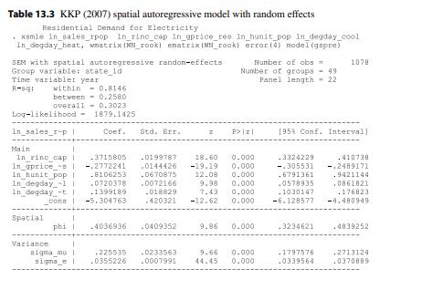
(a) Replicate Tables 13.1, 13.2 and 13.3 using xsmle in Stata showing the maximum likelihood estimates of the Generalized Spatial Panel Random Effects model as well as its special cases of the Anselin and KKP random effects models.

(b) Using the log-likelihood values of these models, test the null that the KKP model restriction is satisfied. Test the null that the Anselin model restriction is satisfied. What do you conclude?

(c) Replicate some of the results in Table 5 of Belotti, Hughes and Piano Mortari (2017). In particular, the first column labeled FE which esimates the residential electricity demand model using fixed effects estimates without any spatial correlation. The second column labeled SAR which estimates a spatial lag model on the dependent variable only. The sixth column labeled SAC, which estimates a SARAR model. The seventh column labeled SEM which estimates a spatial error model as in Anselin (1988), all with fixed effects.

(d) Given the results in part (c), one can use the log-likelihood values to perform the LR tests of Debarsy and Ertur (2010). In particular, you are asked to compute the joint LR test for the spatial lag coefficient \(ho\) as well as the spatial error coefficient \(\lambda\) are zero. This null hypothesis is represented by \(\left(H_{0}^{c}: ho=\lambda=0\right)\) in the text. Also, the marginal LR tests for \(\left(H_{0}^{a}: ho=0\right)\) as well as \(\left(H_{0}^{b}: \lambda=0\right)\). Finally, the conditional LR tests for \(\left(H_{0}^{d}: \lambda=0 / ho\right.\) ) as well as \(\left(H_{0}^{e}: ho=0 / \lambda\right)\). What do you conclude?

(e) Replicate the Spatial Durbin Model (SDM) results given in column 4 of Table 5 of Belotti, Hughes and Piano Mortari (2017). Test the extra spatial Durbin term using the LR test. This can be done by comparing the log-likelihood of SDM with that of SAR.

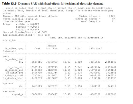
(f) Replicate the dynamic version of the Spatial Durbin Model (dynamic SDM) results given in column 5 of Table 5 of Belotti, Hughes and Piano Mortari (2017). Also, the dynamic version of the Spatial Autoregressive Model (dynamic SAR) results given in column 3 of Table 5 of Belotti, Hughes and Piano Mortari (2017). This is Table 13.5 in this chapter. Test the dynamic terms using the LR test comparing the log-likelihood of SAR with that of dynamic SAR. Also, the LR test comparing SDM with dynamic SDM. Finally, test the spatial Durbin term, as in part

(e) but now for the dynamic model using the LR test comparing the log-likelihood of dynamic SDM with that of dynamic SAR. These LR tests are reported in the first 3 rows of Table 6 of Belotti, Hughes and Piano Mortari (2017). What do you conclude?

(g) Check the sensitivity of the results in part

(f) by adding both the lagged value of the dependent variable and the spatial lag value of the dependent variable with option \(\operatorname{dlag}(3)\) in xsmle. What do you conclude?

image text in transcribed