Reestimate the model in Exercise 9.22 by adding the regressor, expenditure on durable goods.

a. Is there a difference in the regression results you obtained in Exercise 9.22 and in this exercise? If so, what explains the difference?

b. If there is seasonality in the durable goods expenditure data, how would you account for it?

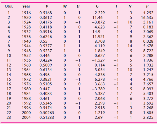
Obs. Year 1916 0.5168 2.229 4.252 1920 0.3612 -11.46 16.535 1924 0.4176 -3.872 -1 10 5.161 -1 4 1928 0.4118 4.623 -1 0.183 1932 0.5916 -1 -14.9 4 7.069 2.362 1936 0.6246 11.921 1940 0.55 3.708 8 0.028 1944 8. 0.5377 4.119 14 5.678 8.722 1948 0.5237 1.849 0.627 10 1952 0.446 6. 2.288 -1.527 11 1956 0.4224 -1 -1 5 1.936 12 1.932 1960 0.5009 0.114 13 1964 0.6134 5.054 10 1.247 1968 1972 0.496 14 4.836 3.215 4.766 7.657 15 0.3821 -1 6.278 -1 4 16 1976 0.5105 3.663 -1 4 17 1980 0.447 -3.789 8.093 18 1984 0.4083 5.387 5.403 19 1988 0.461 2.068 -1 6. 3.272 20 1992 0.5345 2.293 3.692 21 1996 0.5474 2.918 2.268 2000 2004 22 0.50265 1.219 8. 1.605 23 0.51233 1 2.69 -1 2.325 D.