This exercise deals with the loan data in the data file lasvegas described in Exercise 6.18. The "Chow" test was introduced in Section 7.2.3 for testing the equality of coefficients in two regressions on subsets of observations. Here we ask a similar question concerning the parameters of the logit model for delinquency for the two subpopulations of borrowers who either have mortgage insurance \((I N S U R=1)\) or \(\operatorname{not}(I N S U R=0)\).

a. Using all observations, estimate the logit model for DELINQUENT using all explanatory variables except INSUR. Call the value of the log-likelihood function evaluated at the maximum likelihood estimates \(\ln L R\).

b. Reestimate the model in (a) using the sample observations for which \(I N S U R=0\). Call the value of the log-likelihood function evaluated at the maximum likelihood estimates \(\ln L_{0}\).

c. Reestimate the model in (b) using the sample observations for which \(I N S U R=1\). Call the value of the log-likelihood function evaluated at the maximum likelihood estimates \(\ln L_{1}\).

d. Compare the estimates from the models in \((\mathrm{a}-\mathrm{c})\). What major differences in coefficient signs, magnitudes, and significance do you observe?

e. Reestimate the model in (a) including each explanatory variable, as well as INSUR, and its interactions with all the other variables. Compare the value of the log-likelihood function from the fully interacted model, call it \(\ln L_{U}\), to \(\ln L_{0}+\ln L_{1}\). If you have done things correctly, then \(\ln L_{U}\) should equal \(\ln L_{0}+\ln L_{1}\). Can you explain why this must be so?

f. Carry out a likelihood ratio version of the Chow test by computing \(L R=2\left(\ln L_{U}-\ln L_{R}\right)\). What is the appropriate critical value for a test at the \(5 \%\) level of significance? What conclusion do you draw about the subgroups of individuals who do and do not have mortgage insurance? Do the two groups behave in the same way?

Data From Exercise 6.18:-

Consider Example 6.17 where the rice production function
\[\ln (P R O D)=\beta_{1}+\beta_{2} \ln (A R E A)+\beta_{3} \ln (L A B O R)+\beta_{4} \ln (F E R T)+e\]
was estimated using data from the file rice 5.

a. Using data from 1994 only, contrast the outcomes of the following hypothesis tests.

i. \(H_{0}: \beta_{2}=0\) versus \(H_{1}: \beta_{2} eq 0\),
ii. \(H_{0}: \beta_{3}=0\) versus \(H_{1}: \beta_{3} eq 0\),
iii. \(H_{0}: \beta_{2}=\beta_{3}=0\) versus \(H_{1}: \beta_{2} eq 0\) or \(\beta_{3} eq 0\) or both \(\beta_{2}\) and \(\beta_{3}\) are nonzero.

b. Show that the restricted model corresponding to the restriction \(\beta_{2}+\beta_{3}+\beta_{4}=1\) is given by
\[\ln \left(\frac{P R O D}{A R E A}\right)=\beta_{1}+\beta_{3} \ln \left(\frac{L A B O R}{A R E A}\right)+\beta_{4} \ln \left(\frac{F E R T}{A R E A}\right)+e\]

c. Some output from estimating the equation in part (b) using 1994 data is given in Table 6.6. It includes point and interval estimates for \(\beta_{2}, \operatorname{se}\left(b_{2}\right)\), and a \(p\)-value for testing \(H_{0}: \beta_{2}=0\) against \(H_{1}: \beta_{2} eq 0\). Describe how these results can be obtained and verify that they are correct.

d. Estimate a constant-returns-to-scale production function using data from both 1993 and 1994. Compare the standard errors and \(95 \%\) interval estimates with those in Table 6.7 where both years of data were used, but constant returns to scale was not imposed. Include all coefficients in your comparison. What are the auxiliary \(R^{2}\) 's for the two variables in the restricted model?

Data From Example 6.17:-

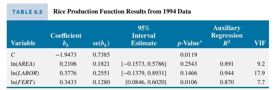
To illustrate collinearity we use data on rice production from a cross section of Philippine rice farmers to estimate the production function 

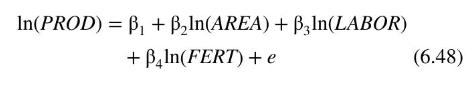
where PROD denotes tonnes of freshly threshed rice, \(A R E A\) denotes hectares planted, \(L A B O R\) denotes person-days of hired and family labor and FERT denotes kilograms of fertilizer. Data for the years 1993 and 1994 can be found in the file rice 5. One would expect collinearity may be an issue. Larger farms with more area are likely to use more labor and more fertilizer than smaller farms. The likelihood of a collinearity problem is confirmed by examining the results in Table 6.5, where we have estimated the function using data from 1994 only. These results convey very little information. The \(95 \%\) interval estimates are very wide, and, because the coefficients of \(\ln (A R E A)\) and \(\ln (L A B O R)\) are not significantly different from zero, their interval estimates include a negative range. The high auxiliary \(R^{2}\) 's and correspondingly high variance inflation factors point to collinearity as the culprit for the imprecise results. Further evidence is a relatively high \(R^{2}=0.875\) from estimating (6.48), and a \(p\)-value of 0.0021 for the joint test of the two insignificant coefficients, \(H_{0}: \beta_{2}=\beta_{3}=0\).

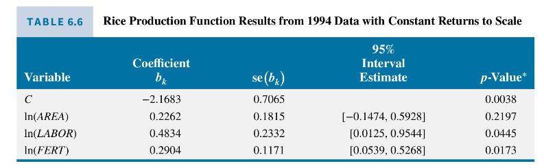
We consider two ways of improving the precision of our estimates: (1) including non-sample information, and (2) using more observations. For non-sample information, suppose that we are willing to accept the notion of constant returns to scale. That is, increasing all inputs by the same proportion will lead to an increase in production of the same proportion. If this constraint holds, then \(\beta_{2}+\beta_{3}+\beta_{4}=1\). Testing this constraint as a null hypothesis yields a \(p\)-value of 0.313 ; so it is not a constraint that is incompatible with the 1994 data. Substituting \(\beta_{2}+\beta_{3}+\beta_{4}=1\) into (6.48) and rearranging the equation gives

\[\begin{equation*}\ln \left(\frac{P R O D}{A R E A}\right)=\beta_{1}+\beta_{3} \ln \left(\frac{L A B O R}{A R E A}\right)+\beta_{4} \ln \left(\frac{F E R T}{A R E A}\right)+e \tag{6.49}\end{equation*}\]
This equation can be viewed as a "yield" equation. Rice yield per hectare is a function of labor per hectare and fertilizer per hectare. Results from estimating it appear in Table 6.6. Has there been any improvement? The answer is not much! The estimate for \(\beta_{3}\) is no longer "insignificant," but that is more attributable to an increase in the magnitude of \(b_{3}\) than to a reduction in its standard error. The reduction in standard errors is only marginal, and the interval estimates are still wide, conveying little information. The squared correlation between \(\ln (\) LABOR/AREA ) and \(\ln\) (FERT/AREA) is 0.414 which is much less than the earlier auxiliary \(R^{2}\) 's, but, nevertheless, the new estimates are relatively imprecise.
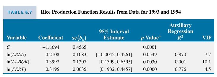
As an alternative to injecting non-sample information into the estimation procedure, we examine the effect of including more observations by combining the 1994 data with observations from 1993. The results are given in Table 6.7. Here there has been a substantial reduction in the standard errors, with considerable improvement in the precision of the estimates, despite the fact that the variance inflation factors still remain relatively large. The greatest improvement has been for the coefficient of \(\ln (F E R T)\), which has the lowest variance inflation factor. The interval estimates for the other two coefficients are still likely to be wider than a researcher would desire, but at least there has been some improvement.

Transcribed Image Text:

In(PROD) = B + ln(AREA) + 3ln(LABOR) +ln(FERT)+e. (6.48)