Question: You are given the data in Table 2.7 for the United States for years 19802006. a. Plot the male civilian labor force participation rate against

You are given the data in Table 2.7 for the United States for years 1980€“2006.

a. Plot the male civilian labor force participation rate against male civilian unemployment rate. Eyeball a regression line through the scatter points. A priori, what is the expected relationship between the two and what is the underlying economic theory? Does the scattergram support the theory?

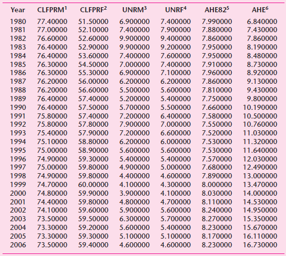
UNRM3 CLFPRM' CLFPRF? UNRF4 АНЕ825 АНЕБ Year 6.840000 7.430000 1980 77.40000 51.50000 6.900000 7.400000 7.400000

b. Repeat (a) for females.
c. Now plot both the male and female labor participation rates against average hourly earnings (in 1982 dollars). (You may use separate diagrams.) Now what do you find? And how would you rationalize your finding?
d. Can you plot the labor force participation rate against the unemployment rate and the average hourly earnings simultaneously? If not, how would you verbalize the relationship among the three variables?

UNRM3 CLFPRM' CLFPRF? UNRF4 825 Year 6.840000 7.430000 1980 77.40000 51.50000 6.900000 7.400000 7.400000 7.900000 7.990000 1981 77.00000 52.10000 7.880000 1982 76.60000 52.60000 9.900000 9.400000 7.860000 7.860000 1983 76.40000 52.90000 9.900000 9.200000 7.950000 8.190000 76.40000 1984 53.60000 7.400000 7.600000 7.950000 8.480000 8.730000 8.920000 1985 7.910000 76.30000 54.50000 7.000000 7.400000 1986 76.30000 55.30000 6.900000 7.100000 7.960000 76.20000 1987 56.00000 6.200000 6.200000 7.860000 9.130000 5.500000 1988 76.20000 56.60000 5.600000 7.810000 9.430000 76.40000 5.400000 1989 57.40000 5.200000 7.750000 9.800000 1990 76.40000 57.50000 5.700000 5.500000 7.660000 10.190000 1991 75.80000 57.40000 7.200000 6.400000 7.000000 7.580000 10.500000 75.80000 1992 57.80000 7.900000 7.550000 10.760000 1993 75.40000 57.90000 7.200000 6.600000 7.520000 11.030000 11.320000 58.80000 1994 75.10000 6.200000 6.000000 7.530000 1995 75.00000 58.90000 5.600000 5.600000 7.530000 11.640000 74.90000 7.570000 12.030000 1996 59.30000 5.400000 5.400000 5.000000 1997 75.00000 59.80000 4.900000 7.680000 12.490000 1998 74.90000 59.80000 4.400000 4.600000 7.890000 13.000000 1999 74.70000 60.00000 4.100000 4.300000 8.000000 13.470000 2000 74.80000 59.90000 3.900000 4.100000 8.030000 14.000000 74.40000 59.80000 2001 4.800000 4.700000 8.110000 14.530000 14.950000 2002 74.10000 59.60000 5.900000 5.600000 8.240000 8.270000 2003 73.50000 59.50000 6.300000 5.700000 15.350000 2004 73.30000 59.20000 5.600000 5.400000 8.230000 15.670000 59.30000 2005 73.30000 5.100000 5.100000 8.170000 16.110000 2006 73.50000 59.40000 4.600000 4.600000 8.230000 16.730000

Step by Step Solution

★★★★★

3.45 Rating (174 Votes )

There are 3 Steps involved in it

1 Expert Approved Answer

Step: 1 Unlock

a The scattergram is as follows The negative relationship between the two variables seems seems rela... View full answer

Question Has Been Solved by an Expert!

Get step-by-step solutions from verified subject matter experts

Step: 2 Unlock

Step: 3 Unlock

Document Format (2 attachments)

1529_605d88e1ca878_656070.pdf

180 KBs PDF File

1529_605d88e1ca878_656070.docx

120 KBs Word File

Students Have Also Explored These Related Econometrics Questions!

You are given the data in Table 6.7. ** Fit the following model to these data and obtain the usual regression statistics and interpret the results: 100 / (100 Y i ) = Î² 1 + Î²...

Given the data in Table 16S-3, what is the probability that the project will be completed in 32 days or less? What is the probability that the project will take longer than 32 days? Task Best Case...

The demand for chicken in the United States, 19601982. To study the per capita consumption of chicken in the United States, you are given the data in the following table, where Y = per capita...

The table gives information reported by the Bureau of Labor Statistics for January 2017. Item Calculate the unemployment rate, the labor force participation rate, and the employment-to-population...

@2 Ram's Furniture Company makes only three kinds of furnitures (chairs, desks and tables). Each product requires some labor in the parts fabrication department, the assembly department and the...

1. Fill in the blanks in the following table: Year Nominal GDP (in billion $) GDP Deflator (2000=100) Real GDP (billions of 2000 $) 1960 526.4 21.04 2,501.8 1970 1,038.5 27.53 1980 2,789.5 5,161.7...

Chap 7 Inflation Video Lecture 41 X QUIZ 5 spring 2022.pdf: ECON10. X QUIZ 5 spring 2022 (1).pdf X + V X C @ File | C:/Users/psdia/Downloads/QUIZ%205%20spring%202022%20(1).pdf G D Apps RD Web Access...

umbers and Graphs: Macroeconomic Measurements, Part I: Prices and Unemployment (Ch 06) Attempts Average / 1 6. Working with Numbers and Graphs Q6 Consider the following data: Population Category...

0 Coastline Home - CCCd edu X '2 Module 8 Labor Markets {Whu X '93 Chapter 13 The Effects of the l\\- x f) ell 6 C plus. pearsonrom Chapter 13 The Effects ofthe Mlnlmurn Wage m GT GD Table Of...

The purpose of your assignment will be to relate the topics covered by the book and discuss whether it is a contradiction or not between being an economist and an ethic/moral aspect of these issues ....

The function h is defined by the power series h(x)= x + 3 x5 x6 +~+~+~+= 7 9 5 xn+2 n=0 2n+1 Part A: Determine the interval of convergence of the power series for h. (10 points) Part B: Find h'(-1)...

What are the similarities between MRP and DRP?

Part A: If the minimum - variance hedge ratio is calculated as 1 . 0 , the hedge must be perfect. Is this statement true or false? Explain. Part B: If there is no basis risk, the minimum variance...

4. Table 1 sets out an economys aggregate demand and aggregate supply schedules. What is the macroeconomic equilibrium? If potential GDP is $600 billion, what is the type of macroeconomic...

Some farmers were interested in predicting inches of growth of corn as a function of rainfall on a monthly basis, so they collected data from the growing season and estimated an equation of the...

In 2001, Heo and Tan published an article in which they used the Granger causality model to test the relationship between economic growth and democracy. For years, political scientists have noted a...

Because their college had just upgraded its residence halls, two seniors decided to build a model of the decision to live on campus. They collected data from 533 upper-class students (first-year...

The Robinson Company has the following current assets and current liabilities for these two years. ________________________________________________________2010______________2011___ Cash and...

Use the approximate doubling time formula (rule of 70) for the case described below. Discuss whether the formula is valid for the case described. Gasoline prices are rising at a rate of 0.3% per...

1. Indicate whether the identifiers below are valid or invalid by putting a () for valid and (x) for invalid. Res num Irvigh 2. Fill in the blanks in each of the following. a) Every C program begins...