In Example 7.9, we conducted a simulation to check the plausibility of the central limit theorem. The variable under consideration there is household size, and the population consists of all U.S. households. A frequency distribution for household size of U.S. households is presented in Table 7.7.

a. Suppose that you simulate 1000 samples of four households each, determine the sample mean of each of the 1000 samples, and obtain a histogram of the 1000 sample means. Would you expect the histogram to be bell-shaped? Explain your answer.

b. Carry out the tasks in part (a) and note the shape of the histogram.

c. Repeat parts (a) and (b) for samples of size 10.

d. Repeat parts (a) and (b) for samples of size 100.

Example 7.9

Household Size According to the U.S. Census Bureau publication Current Population Reports, a frequency distribution for the number of people per household in the United States is as displayed in Table 7.7. Frequencies are in millions of households.

Table 7.7

Here, the variable is household size, and the population is all U.S. households. From Table 7.7, we find that the mean household size is μ = 2.5 persons and the standard deviation is σ = 1.4 persons. Figure 7.5 is a relative-frequency histogram for household size, obtained from Table 7.7. Note that household size is far from being normally distributed; it is right skewed. Nonetheless, according to the central limit theorem, the sampling distribution of the sample mean can be approximated by a normal distribution when the sample size is relatively large. Use simulation to make that fact plausible for a sample size of 30.

Transcribed Image Text:

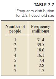
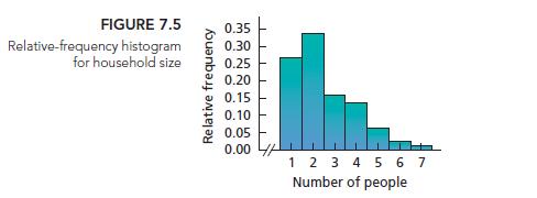
TABLE 7.7 Frequency distribution for U.S. household size Number of Frequency people (millions) 1234567 31.4 39.5 18.6 16.1 7.4 2.8 1.7