Suppose a random sample will be selected from a population that is known to have a normal

Question:

Suppose a random sample will be selected from a population that is known to have a normal distribution. Then the statistic

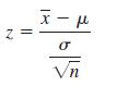
has a standard normal (z) distribution. Since it is rarely the case that σ is known, inferences for population means are usually based on the statistic

which has a t distribution rather than a z distribution. The informal justification for this was that the use of s to estimate σ introduces additional variability, resulting in a statistic whose distribution is more spread out than is the z distribution.

In this activity, you will use simulation to sample from a known normal population, and then investigate how the behavior of

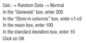
1. Generate 200 random samples of size 5 from a normal population with mean 100 and standard deviation 10. Using MINTAB, go to the Calc Menu. Then

You should now see 200 rows of data in each of the first 5 columns of the MINITAB worksheet.

2. Each row contains five values that have been randomly selected from a normal population with mean 100 and standard deviation 10. Viewing each row as a sample of size 5 from this population, calculate the mean and standard deviation for each of the 200 samples (the 200 rows) by using MINITAB’s row statistics functions, which can also be found under the Calc menu:

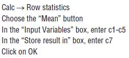
You should now see the 200 sample means in column 7 of the MINITAB worksheet. Name this column “x-bar”, by typing the name in the gray box at the top of c7. Now follow a similar process to compute the 200 sample standard deviations, and store them in c8. Name c8 “s.”

3. Next, calculate the value of the z statistic for each of the 200 samples. We can calculate z in this example because we know that the samples were selected from a population for which σ = 10. Use the calculator function of MINITAB to compute

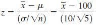
as follows:

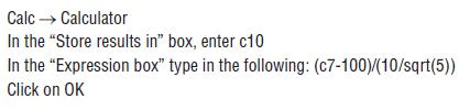
You should now see the z values for the 200 samples in c10. Name c10 “z”.

4. Now calculate the value of the t statistic for each of the 200 samples. Use the calculator function of MINITAB to compute

as follows:

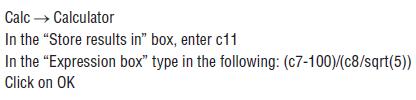
You should now see the t values for the 200 samples in c10. Name c10 “t.”

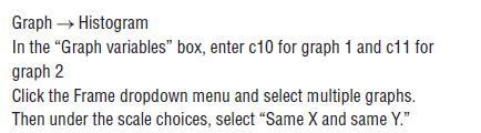
5. Graphs, at last! Now construct histograms of the 200 z values and the 200 t values. These two graphical displays will provide insight about how each of these two statistics behaves in repeated sampling. Use the same scale for the two histograms so that it will be easier to compare the two distributions.

6. Now use the histograms from Step 5 to answer the following questions:

a. Write a brief description of the shape, center and spread for the histogram of the z values. Is what you see in the histogram consistent with what you would have expected to see? Explain.

b. How does the histogram of the t values compare to the z histogram? Be sure to comment on center, shape, and spread.

c. Is your answer to Part (b) consistent with what would be expected for a statistic that has a t distribution? Explain.

d. The z and t histograms are based on only 200 samples, and they only approximate the corresponding sampling distributions. The 5th percentile for the standard normal distribution is −1.645 and the 95th percentile is +1.645. For a t distribution with df = 5 − 1 = 4, the 5th and 95th percentiles are −2.13 and +2.13, respectively. How do these percentiles compare to those of the distributions displayed in the histograms?

e. Are the results of your simulation and analysis consistent with the statement that the statistic