A researcher has 1100 observations on household expenditures on entertainment (per person in the previous quarter, \$) ENTERT. The researcher wants to explain these expenditures as a function of INCOME (monthly income during past year, \$100 units), whether the household lives in an URBAN area, and whether someone in the household has a COLLEGE degree (Bachelor's) or an ADVANCED degree (Master's or Ph.D.). COLLEGE and ADVANCED are indicator variables.

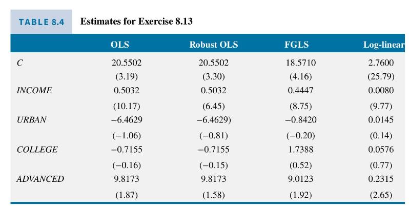
a. The OLS estimates and \(t\)-values are given in Table 8.4, on the next page. Taking the residuals from this regression, and regressing their squared values on all explanatory variables yields an \(R^{2}=0.0344\). Such a small value implies there is no heteroskedasticity, correct? If that statement is not correct, then carry out the proper test. What do you conclude about the presence of heteroskedasticity?

b. To be safe the researcher uses White heteroskedasticity robust standard errors, given in Table 8.4. The researcher's paper has to do with the effect on entertainment expenditures of having someone with an advanced degree in the household. Compare the significance of ADVANCED in the two OLS regressions. What do you find? It is generally true that robust standard errors are larger than ones that are not robust. Is that true or false in this case?

c. Because of the importance of the variable ADVANCED in the model, the researcher takes some additional effort. Using the OLS residuals \(\hat{e}_{i}\), the researcher obtains

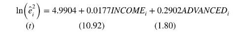
What evidence about heteroskedasticity is present in these results?

d. The researcher takes the results in (c) and then calculates

Each variable, including the intercept, is divided by \(\sqrt{h_{i}}\) and the model reestimated to obtain the FGLS results in Table 8.4. Based on these results, how much of an effect on entertainment expenditures is there for households including someone with an advanced degree? Is this statistically significant? To which set of OLS results, can we make a valid comparison with the FGLS estimates? Have we improved the estimation of the effect of ADVANCED on entertainment by taking the steps in (c) and (d)? Provide a very careful answer to this question.

e. Looking for an easier way the researcher estimates a log-linear model shown in Table 8.4. Following this estimation, regressing the squared residuals on the explanatory variables, we find \(N R^{2}=2.46\). Using White's test, including all the squares and cross-products of the explanatory variables, we obtain \(N R^{2}=6.63\). What are the critical values for each of these test statistics? Using a test at the \(5 \%\) level, do we reject homoskedasticity in the log-linear model or not?

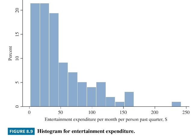
f. Interpret the regression results in (e) from the point of view of the researcher interested in the effect of ADVANCED on entertainment expenditures. What exactly has happened by using the log-linear model? Provide an intuitive explanation. As a hint, Figure 8.9 shows entertainment expenditures for one range of income, between \(\$ 7000 / \mathrm{mo}\) and \(\$ 8000 / \mathrm{mo}\).

Transcribed Image Text:

In () = = 4.9904+0.0177INCOME, +0.2902ADVANCED (t) (10.92) (1.80)