Consider a model for household expenditure as a function of household income using the 2013 data from the Consumer Expenditure Survey, cex5_small. The data file cex5 contains more observations. Our attention is restricted to three person households, consisting of a husband, a wife, plus one other. In this exercise, we examine expenditures on alcoholic beverages.

a. Obtain summary statistics for \(A L C B E V\). How many households spend nothing on alcoholic beverages? Calculate the summary statistics restricting the sample to those households with positive expenditure on alcoholic beverages.

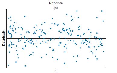
b. Plot \(A L C B E V\) against \(I N C O M E\) and include the fitted least squares regression line. Obtain the least squares estimates of the model \(A L C B E V=\beta_{1}+\beta_{2} I N C O M E+e\). Obtain the least squares residuals and plot these versus INCOME. Does this plot appear random, as in Figure 4.7(a)? If the dependent variable in this regression model is zero \((A L C B E V=0)\), what is the least squares residual? For observations with \(A L C B E V=0\), is the least squares residual related to the explanatory variable INCOME? How?

c. Suppose that some households in this sample may never purchase alcohol, regardless of their income. If this is true, do you think that a linear regression including all the observations, even the observations for which \(A L C B E V=0\), gives a reliable estimate of the effect of income on average alcohol expenditure? If there is estimation bias, is the bias positive (the slope overestimated) or negative (slope underestimated)? Explain your reasoning.

d. For households with \(A L C B E V>0\), construct histograms for \(A L C B E V\) and \(\ln (A L C B E V)\). How do they compare?

e. Create a scatter plot of \(\ln (A L C B E V)\) against \(\ln (I N C O M E)\) and include a fitted regression line. Interpret the coefficient of \(\ln (I N C O M E)\) in the estimated log-log regression. How many observations are included in this estimation?

f. Calculate the least squares residuals from the log-log model. Create a histogram of these residuals and also plot them against \(\ln (I N C O M E\) ). Does this plot appear random, as in Figure 4.7(a)?

g. If we consider only the population of individuals who have positive expenditures for alcohol, do you prefer the linear relationship model, or the log-log model?

h. Expenditures on apparel have some similar features to expenditures on alcoholic beverages. You might reconsider the above exercises for APPAR. Think about part (c) above. Of those with no apparel expenditure last month, do you think there is a substantial portion who never purchase apparel regardless of income, or is it more likely that they sometimes purchase apparel but simply did not do so last month?

Data From Figure 4.7(a):-

Transcribed Image Text:

Residuals x Random (a)