Consider again the data file fred5 used in Example 13.2 and Exercise 13.6.

a. Estimate a VAR model for \(\left\{\Delta C_{t}, \Delta Y_{t}\right\}\) with three lags of each variable included. Comment on the results. Has serial correlation in the errors been eliminated?

b. The concept of "Granger causality" was introduced in Section 9.3.4. In a VAR involving two variables \(x\) and \(y\), we can ask whether \(x\) Granger causes \(y\), whether \(y\) Granger causes \(x\), and whether there is Granger causality in both directions. Using the model estimated in part (a), test whether \(\Delta Y\) Granger causes \(\Delta C\) and whether \(\Delta C\) Granger causes \(\Delta Y\).

Data From Exercise 13.6:-

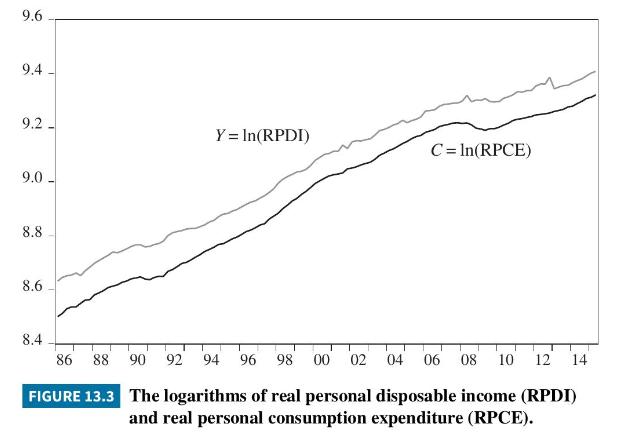
The data file fred 5 contains the \(\log\) of RPDI \((Y)\) and the log of RPCE \((C)\) for the U.S. economy over the period 1986Q1 to 2015Q2.

a. Are the series stationary, or nonstationary? In particular, test whether the series are trend stationary.

b. Test for cointegration allowing for an intercept term. Are the series cointegrated?

c. Estimate a VAR model for the set of \(\mathrm{I}(0)\) variables \(\left\{\Delta C_{t}, \Delta Y_{t}\right\}\). Pay particular attention to the order of lags.

Data From Example 13.2:-

Consider Figure 13.3 that shows the log of real personal disposable income (RPDI) (denoted as \(Y\) ) and the \(\log\) of real personal consumption expenditure (RPCE) (denoted as \(C\) ) for the U.S. economy over the period 1986Q1 to 2015Q2. Both series appear to be nonstationary, but are they cointegrated? The quarterly data are stored in the data file fred5.
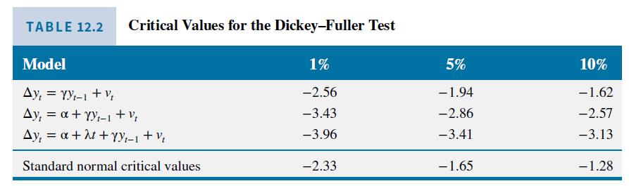
The Dickey-Fuller test values for unit roots for \(C\) were -0.88 when an intercept only was included and -1.63 when both an intercept and trend term were included. In both cases, there were three augmentation terms. The corresponding values for \(Y\) were -1.65 and -0.43 . In these cases, one augmentation term was sufficient. The \(10 \%\) critical values from Table 12.2 are -2.57 without a trend and -3.13 with a trend. Since the test values are greater than the critical values, we cannot conclude that the series are stationary. Using a \(10 \%\) significance level, unit root tests on the first differences of the series lead to a conclusion that the first differences are stationary, and hence the series are I(1). Testing for cointegration yields the following results:

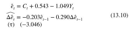
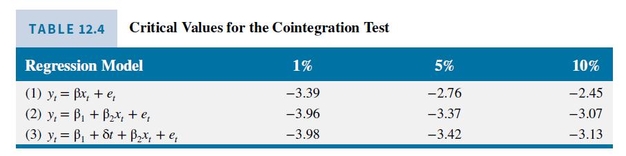
An intercept term has been included to capture the component of \((\log )\) consumption that is independent of disposable income. From Table 12.4, the \(10 \%\) critical value of the test for stationarity in the cointegrating residuals is -3.07 . Since the tau (unit root \(t\)-value) of -3.046 is greater than -3.07 , it indicates that the errors are not stationary and hence that the relationship between \(C\) (i.e., \(\log (\) RPCE)) and \(Y\) (i.e., \(\log (\) RPDI) is spurious. That is, we have no cointegration. Thus, we would not apply a VEC model to examine the dynamic relationship

between aggregate consumption \(C\) and income \(Y\). Instead, we would estimate a VAR model for the set of \(\mathrm{I}(0)\) variables \(\left\{\Delta C_{t}, \Delta Y_{t}\right\}\).
For illustrative purposes, the order of lag in this example has been restricted to one. In general, one should use significance of the coefficient estimates and serial correlation in the errors to choose a suitable number of lags which may be greater than one. The results are

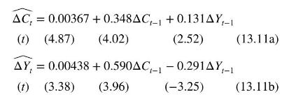
The first equation (13.11a) shows that the quarterly growth in consumption \(\left(\Delta C_{t}\right)\) is significantly related to its own past value \(\left(\Delta C_{t-1}\right)\) and also significantly related to the quarterly growth in last period's income \(\left(\Delta Y_{t-1}\right)\). The second equation (13.11b) shows that \(\Delta Y_{t}\) is significantly negatively related to its own past value but significantly positively related to last period's change in consumption. The constant terms capture the fixed component in the change in log consumption and the change in log income.
Having estimated these models, can we infer anything else? If the system is subjected to an income shock, what is the effect of the shock on the dynamic path of the quarterly growth in consumption and income? Will they rise and by how much? If the system is also subjected to a consumption shock, what is the contribution of an income versus a consumption shock on the variation of income? We turn now to some analysis suited to addressing these questions.

Data From Table 12.2 and 12.4:-

Transcribed Image Text:

, C, +0.543 - 1.049Y, A, = -0.2031 -0.290A-1 (13.10) (T) (-3.046)