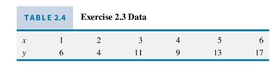
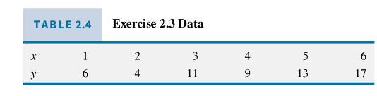
Consider fitting a regression model \(y_{i}=\beta_{1}+\beta_{2} x_{i}+e_{i}\) using the \(N=6\) observations in Table 2.4 from Exercise 2.3, \(\left(y_{i}, x_{i}\right)\). Suppose that based on a theoretical argument we know that \(\beta_{2}=0\).

a. What does the regression model look like, algebraically, if \(\beta_{2}=0\) ?

b. What does the regression model look like, graphically, if \(\beta_{2}=0\) ?

c. If \(\beta_{2}=0\) the sum of squares function becomes \(S\left(\beta_{1}\right)=\sum_{i=1}^{N}\left(y_{i}-\beta_{1}\right)^{2}\). Using the data in Table 2.4, plot the sum of squares function for enough values of \(\beta_{1}\) so that you can locate the approximate minimum. What is this value? [Hint: Your calculations will be easier if you square the term in parentheses and carry through the summation operator.]

d. Using calculus, show that the formula for the least squares estimate of \(\beta_{1}\) in this model is \(\hat{\beta}_{1}=\) \(\left(\sum_{i=1}^{N} y_{i}\right) / N\).

e. Using the data in Table 2.4 and the result in part (d), compute an estimate of \(\beta_{1}\). How does this value compare to the value you found in part (c)?

f. Using the data in Table 2.4, calculate the sum of squared residuals \(S\left(\hat{\beta}_{1}\right)=\sum_{i=1}^{N}\left(y_{i}-\hat{\beta}_{1}\right)^{2}\). Is this sum of squared residuals larger or smaller than the sum of squared residuals \(S\left(b_{1}, b_{2}\right)=\) \(\sum_{i=1}^{N}\left(y_{i}-b_{1}-b_{2} x_{i}\right)^{2}\) using the least squares estimates? [See Exercise 2.3 (d).]

Data From Table 2.4:-

Data From Exercise 2.3:-

Graph the following observations of \(x\) and \(y\) on graph paper.

a. Using a ruler, draw a line that fits through the data. Measure the slope and intercept of the line you have drawn.

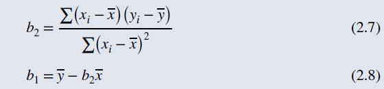
b. Use formulas (2.7) and (2.8) to compute, using only a hand calculator, the least squares estimates of the slope and the intercept. Plot this line on your graph.

c. Obtain the sample means \(\bar{y}=\sum y_{i} / N\) and \(\bar{x}=\sum x_{i} / N\). Obtain the predicted value of \(y\) for \(x=\bar{x}\) and plot it on your graph. What do you observe about this predicted value?

d. Using the least squares estimates from (b), compute the least squares residuals \(\hat{e}_{i}\).

e. Find their sum, \(\sum \hat{e}_{i}\), and their sum of squared values, \(\sum \hat{e}_{i}^{2}\).

f. Calculate \(\sum x_{i} \hat{e}_{i}\).

Data From Formula 2.7 and 2.8:-

Transcribed Image Text:

TABLE 2.4 Exercise 2.3 Data x y 1 6 24 3 11 49 69 17 53 13