Consider the production relationship on Chinese firms used in several chapter examples. We now add another input, MATERIALS. Use the data set from the data file chemical3 for this exercise. (The data file chemical includes many more firms.)

\[\ln \left(\text { SALES }_{i t}\right)=\beta_{1}+\beta_{2} \ln \left(\text { CAPITAL }_{i t}\right)+\beta_{3} \ln \left(\text { LABOR }_{i t}\right)+\beta_{4} \ln \left(\text { MATERIALS }_{i t}\right)+u_{i}+e_{i t}\]

a. Estimate this model using OLS. Compute conventional, heteroskedasticity robust, and cluster-robust standard errors. Using each type of standard error construct a \(95 \%\) interval estimate for the elasticity of SALES with respect to MATERIALS. What do you observe about these intervals?

b. Using each type of standard error in part (a), test at the \(5 \%\) level the null hypothesis of constant returns to scale, \(\beta_{2}+\beta_{3}+\beta_{4}=1\) versus the alternative \(\beta_{2}+\beta_{3}+\beta_{4} eq 1\). Are the results consistent?

c. Use the OLS residuals from (a) and carry out the \(N \times R^{2}\) test from Chapter 9 to test for AR(1) serial correlation in the errors using the 2005 and 2006 data. Is there evidence of serial correlation? What factors might be causing it?

d. Estimate the model using random effects. How do these estimates compare to the OLS estimates? Test the null hypothesis \(\beta_{2}+\beta_{3}+\beta_{4}=1\) versus the alternative \(\beta_{2}+\beta_{3}+\beta_{4} eq 1\). What do you conclude. Is there evidence of unobserved heterogeneity? Carry out the LM test for the presence of random effects at the 5\% level of signficance.

e. Estimate the model using fixed effects. How do the estimates compare to those in (d)? Use the Hausman test for the significance of the difference in the coefficients. Is there evidence that the unobserved heterogeneity is correlated with one or more of the explanatory variables? Explain.

f. Obtain the fixed effects residuals, \(\tilde{e}_{i t}\). Using OLS with cluster-robust standard errors estimate the regression \(\tilde{e}_{i t}=ho \tilde{e}_{i, t-1}+r_{i t}\), where \(r_{i t}\) is a random error. As noted in Exercise 15.10, if the idiosyncratic errors \(e_{i t}\) are uncorrelated we expect \(ho=-1 / 2\). Rejecting this hypothesis implies that idiosyncratic errors \(e_{i t}\) are serially correlated. Using the 5\% level of significance, what do you conclude?

g. Estimate the model by fixed effects using cluster-robust standard errors. How different are these standard errors from the conventional ones in part (e)?

Data From Exercise 15.10:-

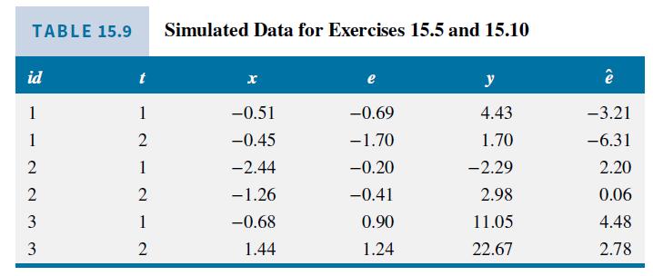
This exercise uses the simulated data \(\left(y_{i t}, x_{i t}\right)\) in Table 15.9.

a. The fitted least squares dummy variable model, given in equation (15.17), is \(\hat{y}_{i t}=5.57 D_{1 i}+\) \(9.98 D_{2 i}+14.88 D_{3 i}+5.21 x_{i t}\). Compute the residuals from this estimated model for \(i d=1\) and \(i d=2\). What pattern do you observe in these residuals?

b. The same residual pattern occurs for \(i d=3\). What is the correlation between the residuals for time periods \(t=1\) and \(t=2\) ?

c. The "within" model is given in equation (15.12). The transformed error is \(\tilde{e}_{i t}=\left(e_{i t}-\bar{e}_{i .}\right)\). If the assumptions FE1-FE5 hold, then \(\operatorname{var}\left(\tilde{e}_{i t}\right)=E\left[\left(e_{i t}-\bar{e}_{i \bullet}\right)^{2}\right]\), where \(\bar{e}_{i \cdot}=\left(e_{i 1}+e_{i 2}\right) / 2\) because \(T=2\). Show that \(\operatorname{var}\left(\tilde{e}_{i t}\right)=\sigma_{e}^{2} / 2\).

d. Using the same approach, as in part (c), show that \(\operatorname{cov}\left(\tilde{e}_{i 1}, \tilde{e}_{i 2}\right)=E\left[\left(e_{i 1}-\bar{e}_{i \text {. }}\right)\left(e_{i 2}-\bar{e}_{i \text {. }}\right)\right]=-\sigma_{e}^{2} / 2\).

e. Using the results in parts (c) and (d), it follows that \(\operatorname{corr}\left(\tilde{e}_{i 1}, \tilde{e}_{i 2}\right)=-1\). Relate this result to your answer in (b). In fact for \(T>1\), and assuming FE1-FE5 hold, \(\operatorname{corr}\left(\tilde{e}_{i t}, \tilde{e}_{i s}\right)=-1 /(T-1)\) if \(t eq s\). We anticipate the within-transformed errors to be serially correlated.

Data From Table 15.9:-

Data From Equation 15.17:-

Transcribed Image Text:

TABLE 15.9 Simulated Data for Exercises 15.5 and 15.10 id t x y 1 -0.51 -0.69 4.43 -3.21 1 2 21212 233 -0.45 -1.70 1.70 -6.31 -2.44 -0.20 -2.29 2.20 -1.26 -0.41 2.98 0.06 -0.68 0.90 11.05 4.48 2 1.44 1.24 22.67 2.78