Example 11.3 introduces Klein's Model I. Here we examine a simplified model that excludes the government sector and allows further practice with simultaneous equations models. Suppose the model is reduced to the following two equations, for two endogenous variables, consumption, \(C N\), and investment, \(I\). The two estimable equations are the consumption and investment functions:

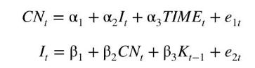
a. Check the identification of the consumption and investment functions.

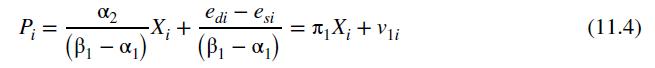
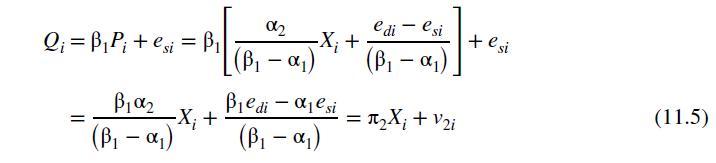
b. Solve for the reduced-form equation for \(C N\). Call the parameters \(\pi_{1}, \pi_{2}, \pi_{3}\) and express them in terms of the structural parameters, similar to equations (11.4) and (11.5).

c. Using the data file klein, estimate each of the structural equations by OLS. Comment on the signs and significance of the coefficients.

d. Estimate each of the structural equations by 2SLS. Comment on the signs and significance of the coefficients.

e. Estimate the first-stage, reduced form, equation. In the reduced-form equation for consumption is \(K_{t-1}\) statistically significant? In the reduced-form equation for investment is \(T I M E_{t}\) statistically significant? Do these results help explain the differences in the OLS and 2SLS estimates?

Data From Equation 11.4 and 11.5:-

Data From Example 11.3:-

One of the most widely used econometric examples in the past 50 years is the small, three equation, macroeconomic model of the U.S. economy proposed by Lawrence Klein, the 1980 Nobel Prize winner in Economics. \({ }^{6}\) The model has three equations, which are estimated, and then a number of macroeconomic identities, or definitions, to complete the model. In all, there are eight endogenous variables and eight exogenous variables.

The first equation is a consumption function, in which aggregate consumption in year \(t, C N_{t}\) is related to total wages earned by all workers, \(W_{t}\). Total wages are divided into wages of workers earned in the private sector, \(W_{1 t}\), and wages of workers earned in the public sector, \(W_{2 t}\), so that total wages \(W_{t}=W_{1 t}+W_{2 t}\). Private sector wages \(W_{1 t}\) are endogenous and determined within the structure of the model, as we will see below. Public sector wages \(W_{2 t}\) are exogenous. In addition, consumption expenditures are related to nonwage income (profits) in the current year, \(P_{t}\), which are endogenous, and profits from the previous year, \(P_{t-1}\). Thus, the consumption function is

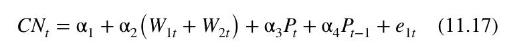
Now refer back to equation (5.44) in Section 5.7.3. There we introduced the term contemporaneously uncorrelated to describe the situation in which an explanatory variable observed at time \(t, x_{t k}\) is uncorrelated with the random error at time \(t, e_{t}\). In the terminology of Chapter 10, the variable \(x_{t k}\) is exogenous if it is contemporaneously uncorrelated with the random error \(e_{t}\). And the variable \(x_{t k}\) is endogenous if it is contemporaneously correlated with the random error \(e_{t}\). In the consumption equation, \(W_{1 t}\) and \(P_{t}\) are endogenous and contemporaneously correlated with the random error \(e_{t}\). On the other hand, wages in the public sector, \(W_{2 t}\), are set by public authority and are assumed exogenous and uncorrelated with the current period random error \(e_{1 t}\). What about profits in the previous year, \(P_{t-1}\) ? They are not correlated with the random error occurring one year later. Lagged endogenous variables are called predetermined variables and are treated just like exogenous variables.
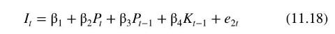
The second equation in the model is the investment equation. Net investment, \(I_{t}\), is specified to be a function of current and lagged profits, \(P_{t}\) and \(P_{t-1}\), as well as the capital stock at the end of the previous year, \(K_{t-1}\). This lagged variable is predetermined and treated as exogenous. The investment equation is

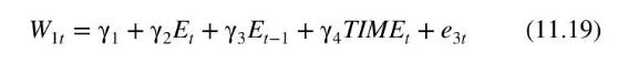
Finally, there is an equation for wages in the private sector, \(W_{1 t}\). Let \(E_{t}=C N_{t}+I_{t}+\left(G_{t}-W_{2 t}\right)\), where \(G_{t}\) is government spending. Consumption and investment are endogenous and government spending and public sector wages are exogenous. The sum, \(E_{t}\), total national product minus public sector wages, is endogenous. Wages are taken to be related to \(E_{t}\) and the predetermined variable \(E_{t-1}\), plus a time trend variable, TIME \(_{t}=\) YEAR \(_{t}-1931\), which is exogenous. The wage equation is

Because there are eight endogenous variables in the entire system there must also be eight equations. Any system of \(M\) endogenous variables must have \(M\) equations to be complete. In addition to the three equations (11.17)-(11.19), which contain five endogenous variables, there are five other definitional equations to complete the system that introduce three further endogenous variables. In total, there are eight exogenous and predetermined variables, which can be used as IVs. The exogenous variables are government spending, \(G_{t}\), public sector wages, \(W_{2 t}\), taxes, \(T X_{t}\), and the time trend variable, TIME . Another exogenous variable is the constant term, the "intercept" variable in each equation, \(X_{1 t} \equiv 1\). The predetermined variables are lagged profits, \(P_{t-1}\), the lagged capital stock, \(K_{t-1}\), and the lagged total national product minus public sector wages, \(E_{t-1}\).

Data From Equation 5.44:-

Transcribed Image Text:

CN = +1, +3TIME, + et IB+BCN, B3 K1 + e 21