Examples 15.7 and 15.8 estimate a production function by OLS and fixed effects, respectively, with both conventional nonrobust standard errors and cluster-robust standard errors for \(N=1000\) Chinese chemical firms for 2004-2006.

a. Review the examples. What is the percent difference between the cluster-robust standard errors and the conventional standard errors?

b. Let \(\hat{v}_{i t}\) denote the OLS residuals from Example 15.7 and let \(\hat{v}_{i, t-1}\) be the lagged residuals. Consider the regression \(\hat{v}_{i t}=ho \hat{v}_{i, t-1}+r_{i t}\), where \(r_{i t}\) is an error term. Regressing the 2006 residuals on the 2005 residuals, we obtain \(\hat{ho}=0.948\) with conventional OLS standard error 0.017 and White heteroskedasticity-consistent standard error 0.020 . Do these results establish a time-series serial correlation in the idiosyncratic error component \(e_{i t}\) ? If not, what is the source of the strong correlation between \(\hat{v}_{i t}\) and \(\hat{v}_{i, t-1}\) ?

c. Let \(\hat{\tilde{e}}_{i t}\) be the residuals from the within estimation, similar to Example 15.5, but using all 1000 firms. Let \(\hat{\tilde{e}}_{i, t-1}\) be the lagged residuals. As noted in Exercise 15.10, part (e), we expect the errors in the "within" transformed model to be serially correlated with correlation \(\operatorname{corr}\left(\tilde{e}_{i t} \tilde{e}_{i s}\right)=-1 /(T-1)\) under FE1-FE5. Here \(T=3\), thus we should find \(\operatorname{corr}\left(\tilde{e}_{i t} \tilde{e}_{i s}\right)=-1 / 2\). Consider the regression \(\hat{\tilde{e}}_{i t}=ho \hat{\tilde{e}}_{i, t-1}+r_{i t}\), where \(r_{i t}\) is an error term. Using the 2006 data and \(N=1000\) observations, we estimate the value of \(ho\) to be -0.233 with conventional standard error 0.046 , and White heteroskedasticity robust standard error of 0.089 . Test the null hypothesis \(ho=-1 / 2\) against the alternative \(ho eq-1 / 2\) using a \(t\)-test at the \(5 \%\) level, first with the conventional standard error and again with the heteroskedasticity robust standard error. Rejecting the null hypothesis implies that FE4, part (ii), does not hold, and time-series serial correlation exists in the idiosyncratic errors \(e_{i t}\). Such a finding justifies the use of cluster-robust standard errors in the fixed effects model regardless of any heteroskedasticity considerations.

d. Using the \(N=2000\) observations for 2005-2006, and the estimated regression \(\hat{\tilde{e}}_{i t}=ho \hat{\tilde{e}}_{i, t-1}+\) \(r_{i t}\), we estimate the value of \(ho\) to be -0.270 with cluster-robust standard error, suggested by Wooldridge (2010, p. 311), of 0.017 . Test the null hypothesis \(ho=-1 / 2\) against the alternative \(ho eq-1 / 2\) using a \(t\)-test at the \(5 \%\) level. Rejecting the null hypothesis implies that FE4, part (ii), does not hold, and time-series serial correlation exists in the idiosyncratic errors \(e_{i t}\).

Data From Example 15.7:-

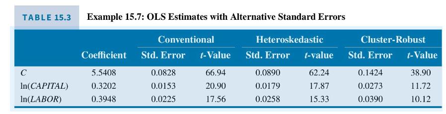
In Example 15.6, we found that there is strong evidence in favor of using the fixed effects estimator rather than the pooled OLS estimator using the Chinese chemical firm data. However, for the purpose of giving a numerical illustration of pooled OLS with and without clustering, we examine the baseline model in Example 15.2 using \(N=1000\) firms using data file chemical3. Table 15.3 shows the OLS estimates with conventional, heteroskedasticity robust, and clusterrobust standard errors, and \(t\)-statistic values.
Note that while the heteroskedasticity-corrected standard errors are larger than the conventional standard errors, the cluster-corrected standard errors are larger yet. Of course, the \(t\)-values become smaller with the increased standard errors.

Data From Example 15.6:-

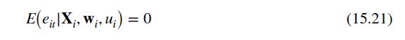
For the Chinese chemical firm data file chemical2, the indicator variable model in (15.21) becomes
\[\begin{aligned}\ln \left(\text { SALES }_{i t}\right)= & \beta_{11} D_{1 i}+\cdots+\beta_{1,200} D_{200, i}+\beta_{2} \ln \left(\text { CAPITAL }_{i t}\right) \\& +\beta_{3} \ln \left(\text { LABOR }_{i t}\right)+e_{i t}\end{aligned}\]
The fixed effects estimates of \(\beta_{2}\) and \(\beta_{3}\) will be identical to the within estimates in Example 15.4, and the standard errors will be the correct ones because in this indicator variable model the degrees of freedom are the correct \(N T-N-(K-1)=\) \(600-200-2=398\).
The \(N=200\) estimated indicator variable coefficients, \(b_{11}, b_{12}, \ldots, b_{1 N}\), may or may not be of specific interest. We include the indicator variables primarily to control for unobserved heterogeneity. If, however, we are interested in predicting the sales of a specific firm then the indicator variables become crucial. Given the estimates of \(\beta_{2}\) and \(\beta_{3}, b_{11}, b_{12}, \ldots\), \(b_{1 N}\) can be recovered using the fact that the fitted regression passes through the point of the means, just as it did in the simple regression model, that is, \(\bar{y}_{i .}=b_{1 i}+b_{2} \bar{x}_{2 i .}+b_{3} \bar{x}_{3 i}\), \(i=1, \ldots, N\). Reporting the estimates and their standard errors is inconvenient because \(N\) may be large. Software companies cope with this in different ways. Two popular econometric software programs, EViews and Stata, report a constant term \(C\) that is the average of the estimated coefficients on the cross-section indicator variables. For the Chinese chemical firm data, \(C=N^{-1} \sum_{i=1}^{N} b_{1 i}=7.5782\).
To test the null hypothesis \(H_{0}: \beta_{11}=\beta_{12}, \beta_{12}=\beta_{13}, \ldots\), \(\beta_{1, N-1}=\beta_{1 N}\), we use the sum of squared residuals from the fixed effects estimator, \(S S E_{U}=34.451469\), and from the pooled OLS regression

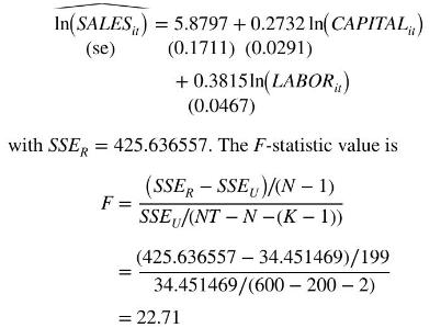
Using the \(\alpha=0.01\) level of significance, \(F_{(0.99,199,398)}=1.32\). We reject the null hypothesis and conclude that there are individual differences in the fixed effects constant terms for these \(N=200\) firms.

Data From Equation 15.21:-

Data From Example 15.2:-

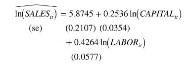
The data file chemical2 contains data on \(N=200\) chemical firms' sales in China for the years 2004-2006. We wish to estimate the log-log model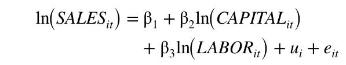

Using only data from 2005 and 2006, the OLS estimates with conventional, nonrobust, standard errors are

We may be concerned that there are unobserved individual differences among the firms that are correlated with their usage of capital and labor in the production and sales process. The estimated first-difference model is

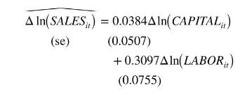
There is a remarkable reduction in the estimated effect of the capital stock, which is no longer statistically significant. The estimated effect of labor is smaller but still significantly different from zero. The difference estimator is consistent when unobserved heterogeneity is correlated with the explanatory variables, but the OLS estimator is not. Given the substantial difference in the estimates we might suspect that the OLS estimates are unreliable.

Data From Example 15.8:-

In Example 15.7, we estimated the production function by OLS with alternative standard errors. Here using data file chemical3, we obtain the fixed effects estimates using \(N=1000\) firms with conventional standard errors and cluster-robust standard errors. The cluster-robust standard errors are substantially larger than the usual standard errors. When this is the case, using the cluster-robust standard errors is recommended if \(N\) is large and \(T\) is small, like they are in this case (Table 15.4).

Transcribed Image Text:

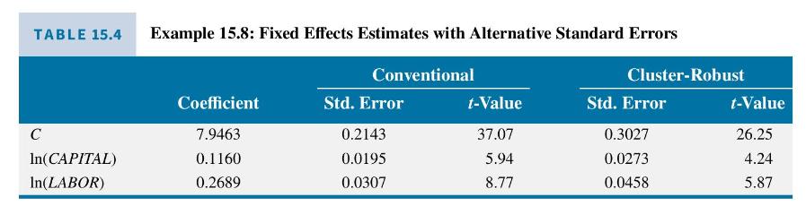
TABLE 15.3 Example 15.7: OLS Estimates with Alternative Standard Errors Conventional Heteroskedastic Cluster-Robust Coefficient Std. Error t-Value Std. Error t-value Std. Error t-Value C 5.5408 0.0828 66.94 0.0890 62.24 0.1424 38.90 In(CAPITAL) 0.3202 0.0153 20.90 0.0179 17.87 0.0273 11.72 In(LABOR) 0.3948 0.0225 17.56 0.0258 15.33 0.0390 10.12