In Example 16.3, we illustrate the calculation of the likelihood function for the probit model in a small example.

a. Calculate the probability that \(y=1\) if \(x=1.5\), given the values of the maximum likelihood estimates.

b. Using the threshold 0.5 and the result in part (a), predict the value of \(y\) if \(x=1.5\), the first observation, given the values of the maximum likelihood estimates. Does your prediction agree with the actual outcome \(y=1\) ?

c. Calculate the value of the likelihood function, illustrated in equation (16.14), using the given \(N=3\) data pairs, if the parameter values are \(\beta_{1}=-1\) and \(\beta_{2}=0.2\). Compare this value to the value of the likelihood function evaluated at the maximum likelihood estimates, given in Example 16.3. Which is larger?

d. For the probit model, the value of the likelihood function (16.14) will always be between zero and one. True or false? Explain.

e. For the probit model, the value of the log-likelihood function (16.15) will always be negative. True or false? Explain.

Data From Example 16.3:-

We first illustrate the idea of maximum likelihood estimation in an abbreviated version of the transportation choice model from Examples 16.1 and 16.2. Suppose that we randomly select three individuals and observe that the first two drive to work and the third takes the bus; \(y_{1}=1, y_{2}=1, y_{3}=0\). Furthermore, suppose that the differences in commuting times for these individuals, in 10-minute units, are \(x_{1}=1.5\), \(x_{2}=0.6, x_{3}=0.7\). What is the joint probability of observing \(y_{1}=1, y_{2}=1, y_{3}=0\) ? The probability function for \(y_{i}\) is given by (16.2), which we now combine with the probit model (16.10) to obtain
\[\begin{aligned}& f\left(y_{i} \mid x_{i}\right) \\& \quad=\left[\Phi\left(\beta_{1}+\beta_{2} x_{i}\right)\right]^{y_{i}}\left[1-\Phi\left(\beta_{1}+\beta_{2} x_{i}\right)\right]^{1-y_{i}}, \quad y_{i}=0,1\end{aligned}\]
If the three individuals are independently drawn, then the joint \(p d f\) for \(y_{1}, y_{2}\), and \(y_{3}\) is the product of the marginal probability functions:
\[f\left(y_{1}, y_{2}, y_{3} \mid x_{1}, x_{2}, x_{3}\right)=f\left(y_{1} \mid x_{1}\right) f\left(y_{2} \mid x_{2}\right) f\left(y_{3} \mid x_{3}\right)\]

Consequently, the probability of observing \(y_{1}=1, y_{2}=1\), and \(y_{3}=0\) is
\[\begin{aligned}& P\left(y_{1}=1, y_{2}=1, y_{3}=0 \mid x_{1}, x_{2}, x_{3}\right) \\& \quad=f\left(1,1,0 \mid x_{1}, x_{2}, x_{3}\right)=f\left(1 \mid x_{1}\right) f\left(1 \mid x_{2}\right) f\left(0 \mid x_{3}\right)\end{aligned}\]

Substituting the \(y\) and \(x\) values, we have

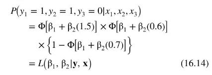
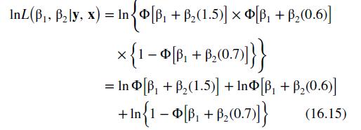
or likelihood, of the observed outcome. Unfortunately, for the probit model, there are no formulas that give us the values for \(\tilde{\beta}_{1}\) and \(\tilde{\beta}_{2}\) as there are in least squares estimation of the linear regression model. Consequently, we must use the computer and techniques from numerical analysis to find the values \(\tilde{\beta}_{1}\) and \(\tilde{\beta}_{2}\) that maximize \(L\left(\beta_{1}, \beta_{2} \mid \mathbf{y}, \mathbf{x}\right)\). In practice, instead of maximizing (16.14), we maximize the logarithm of (16.14), which is called the log-likelihood function

On the surface, this appears to be a difficult task, because \(\Phi(z)\) from (16.9) is such a complicated function. As it turns out, however, using a computer to maximize (16.15) is a relatively easy process.

The maximization of the log-likelihood function \(\ln L\left(\beta_{1}, \beta_{2} \mid \mathbf{y}, \mathbf{x}\right)\) is easier than the maximization of (16.14), because it is a sum of terms and not a product of terms. The logarithm is a nondecreasing, or monotonic, function so that the maximum values of the two functions \(L\left(\beta_{1}, \beta_{2} \mid \mathbf{y}, \mathbf{x}\right)\) and \(\ln L\left(\beta_{1}, \beta_{2} \mid \mathbf{y}, \mathbf{x}\right)\) occur at the same values of \(\beta_{1}\) and \(\beta_{2}\), namely, \(\tilde{\beta}_{1}\) and \(\tilde{\beta}_{2}\). The value of the log-likelihood function (16.15) evaluated at the maximizing values \(\tilde{\beta}_{1}\) and \(\tilde{\beta}_{2}\) is very useful for hypothesis testing, which is discussed in Sections 16.2.4 and 16.2.5. Using econometric software, we find that the parameter values that maximize (16.15) are \(\tilde{\beta}_{1}=-1.1525\) and \(\tilde{\beta}_{2}=0.1892\). These values maximize the log-likelihood function, \(\ln L\left(\beta_{1}, \beta_{2} \mid \mathbf{y}, \mathbf{x}\right)\), and also maximize the likelihood function \(L\left(\beta_{1}, \beta_{2} \mid \mathbf{y}, \mathbf{x}\right)\). They are the maximum likelihood estimates. Any other values of the parameters that we might try will yield a lower value of the log-likelihood function. Plugging these values into (16.15), we obtain the value of the log-likelihood function evaluated at the maximum likelihood estimates, which is \(L\left(\tilde{\beta}_{1}, \tilde{\beta}_{2} \mid \mathbf{y}, \mathbf{x}\right)=-1.5940\).

Data From Example 16.1:-

An important problem in transportation economics is explaining an individual's choice between driving (private transportation) and taking the bus (public transportation) when commuting to work, assuming, for simplicity, that these are the only two alternatives. We can imagine many factors that affect the choice, including an individual's characteristics, such as age, income, and sex; the characteristics of their automobile, such as its reliability, comfort, and fuel economy; the characteristics of the public transportation, such as reliability, cost, and safety. In our example, we will focus on a single factor, commuting time. Define the explanatory variable
\[x_{i}=\text { (commuting time by bus }\]
- commuting time by car, for the \(i\) th individual)
A priori we expect that as \(x_{i}\) increases, and commuting time by bus increases relative to commuting time by car, and holding all else constant, an individual would be more inclined to drive. Suppose that alternative one is driving to work, \(y_{i}=1\), and alternative two is taking public transportation, \(y_{i}=0\). Then the probability that the \(i\) th individual drives to work is \(P\left(y_{i}=1 \mid x_{i}\right)=p\left(x_{i}\right)\). Our reasoning suggests that there is a positive relationship between the difference in commuting time and the probability that an individual will drive to work. Using data on individuals and their choices, we will obtain estimates of how much increases in commuting time by bus relative to driving will affect the probability that an individual will drive. Using the estimates, we can predict the choice of an individual when the commuting time by bus is, for example, 20 minutes longer than the commuting time by car. We will also develop methods for testing hypotheses about the nature of the relationship, such as testing whether the difference in commuting time is a statistically significant factor in the decision.

Data From Example 16.2:-

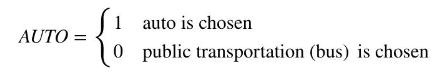
Ben-Akiva and Lerman \({ }^{1}\) have sample data on automobile and public transportation travel times and the alternative chosen for \(N=21\) individuals in the data file transport. The variable \(A U T O\) is an indicator variable taking the value one if automobile transportation is chosen and is zero if public transportation is chosen,

The variables AUTOTIME and BUSTIME are minutes of commuting time. The explanatory variable we consider is DTIME \(=(\) BUSTIME - AUTOTIME \() \div 10\), which is the commuting time differential in 10 -minute increments. The linear probability model is AUTO \(_{i}=\beta_{1}+\beta_{2}\) DTIME \(_{i}+e_{i}\). The OLS fitted model, with heteroskedasticity robust standard errors, is
\[\begin{array}{lll}\widehat{A U T O}_{i}=0.4848+0.0703 D T I M E_{i} & R^{2}=0.61 \\\text { (robse) } \quad(0.0712)(0.0085) &\end{array}\]
We estimate that if travel times by public transportation and automobile are equal, so that DTIME \(=0\), then the probability of a person choosing automobile travel is 0.4848 , close to \(50-50\), with a \(95 \%\) interval estimate of [0.34, 0.63]. We estimate that, holding all else constant, an increase of 10 minutes in the difference in travel time, increasing public transportation travel time relative to automobile travel time, increases the probability of choosing automobile travel by 0.07 , with a \(95 \%\) interval estimate of \([0.0525,0.0881]\), which seems relatively precise. In truth, any judgment about precision depends on the use to which the results will be put. The fitted model can be used to estimate the probability of automobile travel for any commuting time differential. For example, if \(D T I M E=1\), a 10-minute longer commute by public transportation, we estimate the probability of automobile travel to be \(\widehat{A U T O}_{i}=0.4848+0.0703(1)=0.5551\).
How well does the model fit the data? The \(R^{2}=0.61\) suggests that \(61 \%\) of the variation in the outcome variable is explained by the model. With probability models, we can examine how well the model predicts the outcomes. Let's predict the choice using a probability threshold of 0.50 . That is, if \(\widehat{A U T O}_{i} \geq 0.50\) we predict that a person will drive to work, and otherwise, we predict that a person will use public transportation. In the sample of 21 individuals, 10 drove to work and 11 used public transportation. Using the classification rule, we successfully predict 9 of the 10 drivers, and 10 of the 11 bus riders. That is 19 successful predictions out of the 21 cases. Looking at individual estimated probabilities of driving, we find three negative values. If the commute is 69 minutes or less by public transportation, then the estimated probability of driving is zero or negative. If commuting time is 73 minutes or more by public transportation, then the estimated probability of driving is one or greater.

Data From Equation 16.15 and 16.2:-

Transcribed Image Text:

P(y = 1, y2 = 1, y3 = 0x1, x2, x3) = [, + (1.5)] [ + (0.6)] x{1-B,+P(0.7)]} = L(B1, Bly, x) (16.14)