

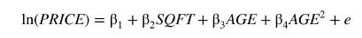
Question: In Example 6.18, using 900 observations from the data file (b r 5), we identified three potentially influential observations in the estimation of the model
In Example 6.18, using 900 observations from the data file \(b r 5\), we identified three potentially influential observations in the estimation of the model
![]()
Those observations were numbers 150,411 and 540.
a. Estimate the model with (i) all observations, (ii) observation 150 excluded, (iii) observation 411 excluded, (iv) observation 540 excluded, and (v) observations 150, 411, and 540 excluded. Report the results and comment on their sensitivity to the omission of the observations.
b. Using the estimates from all observations, find the forecast errors corresponding to the within sample predictions at observations 150,411 , and 540.
c. Using the estimates obtained when observation 150 is excluded, find the out-of-sample forecast error for observation 150 .
d. Using the estimates obtained when observation 411 is excluded, find the out-of-sample forecast error for observation 411.
e. Using the estimates obtained when observation 540 is excluded, find the out-of-sample forecast error for observation 540.
f. Using the estimates obtained when observations 150,411 , and 540 are excluded, find the out-of-sample forecast errors for observations 150, 411, and 540.
g. Compare the forecast errors obtained in parts (b)- (f) and comment on their sensitivity to the omission of the observations.
Data From Example 6.18:-
To illustrate the identification of potentially influential observations, we return to Example 6.16 where, using predictive model selection criteria, the preferred equation for predicting house prices was
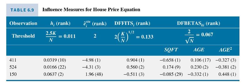
In a sample of 900 observations it is not surprising to find a relatively large number of data points where the various influence measures exceed the recommended thresholds. As examples, in Table 6.9 we report the values of the measures for those observations with the three largest DFFITS. It turns out that the other influence measures for these three observations also have large values. In parentheses next to each of the values is the rank of its absolute value. When we check the characteristics of the three unusual observations, we find observation 540 is the newest house in the sample and observation 150 is the oldest house. Observation 411 is both old and large; it is the 10th largest (99th percentile) and the sixth oldest (percentile 99.4) house in the sample. In Exercise 6.20, you are invited to explore further the effect of these observations.
Data From Example 6.16:-
Real estate agents and potential homebuyers are interested in valuing houses or predicting the price of a house with particular characteristics. There are many factors that have a bearing on the price of a house, but for our predictive model we will consider just two, the age of the house in years (AGE), and its size in hundreds of square feet (SQFT). The most general model we consider is
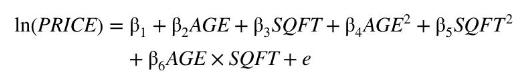
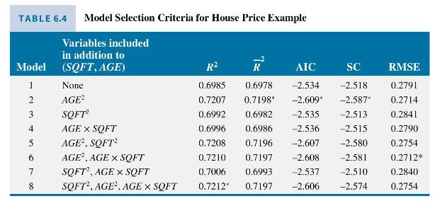
where PRICE is the house price in thousands of dollars. Of interest is whether some or all of the quadratic terms \(A G E^{2}\), \(S Q F T^{2}\), and \(A G E \times S Q F T\) improve the predictive ability of the model. For convenience, we evaluate predictive ability in terms of \(\ln (\) PRICE) not PRICE. We use data on 900 houses sold in Baton Rouge, Louisiana in 2005, stored in the data file br5. For a comparison based on the RMSE of predictions (but not the other criteria) we randomly chose 800 observations for estimation and 100 observations for the hold-out sample. After this random selection, the observations were ordered so that the first 800 were used for estimation and the last 100 for predictive assessment. Values of the criteria for the various models appear in Table 6.4. Looking for the model with the highest \(\bar{R}^{2}\), and the models with the smallest values (or largest negative numbers) for the AIC and SC, we find that all three criteria prefer model 2 where \(A G E^{2}\) is included, but \(S Q F T^{2}\) and \(A G E \times S Q F T\) are excluded. Using the out-of-sample RMSE criterion, model 6 , with \(A G E \times S Q F T\) included in addition to \(A G E^{2}\), is slightly favored over model 2.
In(PRICE) B+ B2SQFT+ B3AGE + BAGE
Step by Step Solution
There are 3 Steps involved in it
StepbyStep Solution Part a Model Estimations with Selected Observations Excluded To estimate the models we need to perform multiple regressions as described 1 All Observations Perform regression using ... View full answer

Get step-by-step solutions from verified subject matter experts