

Reconsider Example 6.20 where a logistic growth curve for the share of U.S. steel produced by electric
Question:
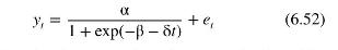
Reconsider Example 6.20 where a logistic growth curve for the share of U.S. steel produced by electric arc furnace (EAF) technology was estimated. The curve is given by the equation
a. Find \(95 \%\) interval estimates for the following:
i. The saturation level \(\alpha\).
ii. The inflection point \(t_{I}=-\beta / \delta\) at which the rate of growth starts to decline. What years does the interval correspond to?
iii. The EAF share in 1969.
iv. The predicted EAF shares from 2016 to 2050. Plot the predictions and their \(95 \%\) bounds. Comment on how far the predictions are from the saturation level and on the behavior of the \(95 \%\) bounds.
b. Use a 5\% significance level to test the joint null hypothesis that the saturation level is 0.85 and the point of inflection is at \(t_{I}=25\). Set up the null hypothesis for the point of inflection so that it is linear in the parameters \(\beta\) and \(\delta\). Given the interval estimates you found in (a)(i) and (a)(ii), does the result surprise you? What extra information does the test use that was not used in (a)(i) and (a)(ii)?
c. Estimate the model with the restrictions implied by the null hypothesis in (b) imposed. Find the sum of squared errors and test the null hypothesis with an \(F\)-test that uses the restricted and unrestricted sums of squared errors. How does this result compare with that from the automatic test command that you used for part (b)?
Data From Example 6.20:-
A model that is popular for modeling the diffusion of technological change is the logistic growth curve \({ }^{13}\)
where \(y_{t}\) is the adoption proportion of a new technology. For example, \(y_{t}\) might be the proportion of households who own a computer, or the proportion of computer-owning households who have the latest computer, or the proportion of musical recordings sold as compact disks. In the example that follows, \(y_{t}\) is the share of total U.S. crude steel production that is produced by electric arc furnace technology.
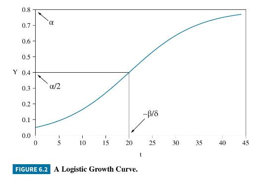
Before considering this example, we note some details about the relationship in equation (6.52). There is only one explanatory variable on the right hand side, namely, time, \(t=1,2, \ldots, T\). Thus, the logistic growth model is designed to capture the rate of adoption of technological change, or, in some examples, the rate of growth of market share. An example of a logistic curve is depicted in Figure 6.2. In this example, the rate of growth increases at first, to a point of inflection that occurs at \(t=-\beta / \delta=20\). Then the rate of growth declines, leveling off to a saturation proportion given by \(\alpha=0.8\). Since \(y_{0}=\alpha /(1+\exp (-\beta))\), the parameter \(\beta\) determines how far the share is below saturation level at time zero. The parameter \(\delta\) controls the speed at which the
point of inflection, and the saturation level, are reached. The curve is such that the share at the point of inflection is \(\alpha / 2=0.4\), half the saturation level.
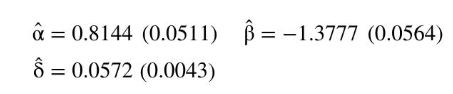
Traditional technology for steel making, involving blast and oxygen furnaces and the use of iron ore, is being displaced by newer electric arc furnace technology that utilizes scrap steel. This displacement has implications for the suppliers of raw materials such as iron ore. Thus, prediction of the future electric arc furnace share of steel production is of vital importance to mining companies. The file steel contains annual data on the electric arc furnace share of U.S. steel production from 1970 to 2015. Using this data to find nonlinear least squares estimates of a logistic growth curve yields the following estimates (standard errors):
Quantities of interest are the inflection point at which the rate of growth of the share starts to decline, \(-\beta / \delta\); the saturation proportion \(\alpha\); the share at time zero, \(y_{0}=\alpha /(1+\exp (-\beta))\); and prediction of the share for various years in the future. In Exercise 6.21, you are invited to find interval estimates for these quantities.
Step by Step Answer:

This question has not been answered yet.
You can Ask your question!


Principles Of Econometrics
ISBN: 9781118452271
5th Edition
Authors: R Carter Hill, William E Griffiths, Guay C Lim
