In Example 9.13, the following finite distributed lag model was estimated for Okun's Law using the data file okun5_aus.

a. Find the correlogram of the least squares residuals for this model. Is there any evidence of autocorrelation?

b. Test for autocorrelation in the residuals using the \(\chi^{2}=T \times R^{2}\) version of the LM test, with missing initial values for \(\hat{e}_{t}\) set to zero, and lags up to 4. Is there any evidence of autocorrelation?

c. Compare \(95 \%\) interval estimates for the coefficients obtained using conventional OLS standard errors with those obtained using HAC standard errors.

Data From Example 9.13:-

To illustrate the various distributed lag concepts, we introduce an economic model known as Okun's Law. \({ }^{10}\) In this model, we again consider a relationship between unemployment and growth of the economy, but we formulate the model differently and use a different data set. Moreover, our purpose is not to forecast unemployment but to investigate the lagged responses of unemployment to growth in the economy. In the basic model for Okun's Law, the change in the unemployment rate from one period to the next depends on the rate of growth of output in the economy:

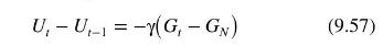
where \(U_{t}\) is the unemployment rate in period \(t, G_{t}\) is the growth rate of output in period \(t\), and \(G_{N}\) is the "normal" growth rate, which we assume is constant over time. The parameter \(\gamma\) is positive, implying that when the growth of output is above the normal rate, unemployment falls; a growth rate below the normal rate leads to an increase in unemployment. The normal growth rate \(G_{N}\) is the rate of output growth needed to maintain a constant unemployment rate. It is equal to the sum of labor force growth and labor productivity growth. We expect \(0
To write (9.57) in the more familiar notation of the multiple regression model, we denote the change in

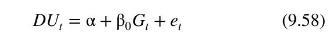
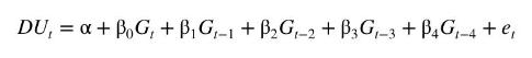
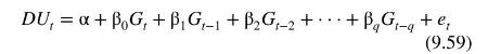
Recognizing that changes in output are likely to have a distributed-lag effect on unemployment-not all of the effect will take place instantaneously-we expand (9.58) to include lags of \(G_{t}\)

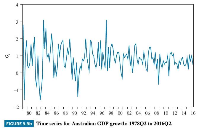
To estimate this relationship, we use quarterly Australian data on unemployment and the percentage change in gross domestic product (GDP) from quarter 2, 1978 to quarter 2, 2016. These data are stored in the file okun5_aus. The time series for \(D U\) and \(G\) are graphed in Figure 9.9(a) and (b). There are noticeable jumps in the unemployment rate around 1983, 1992, and 2009; they correspond roughly to periods when there was negative growth but with a lag. At this time, we also note that the series appear to be stationary; tools for more rigorous assessment of stationarity are deferred until Chapter 12.
Least squares estimates of the coefficients and related statistics for equation (9.59) are reported in Table 9.7 for lag

lengths \(q=4\) and \(q=5\). All coefficients of \(G\) and its lags have the expected negative sign and are significantly different from zero at a 5\% significance level, with the exception of that for \(G_{t-5}\) when \(q=5\). Given the coefficient of this lag is positive

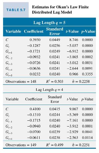
and insignificant, we drop \(G_{t-5}\) and settle on a model of order \(q=4\) where all coefficients have the expected negative signs and are significantly different from zero.
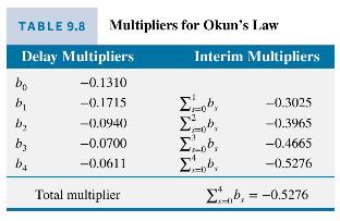
What do the estimates for lag length 4 tell us? A 1\% increase in the growth rate leads to a fall in the expected unemployment rate of \(0.13 \%\) in the current quarter, a fall of \(0.17 \%\) in the next quarter and falls of \(0.09 \%, 0.07 \%\), and \(0.06 \%\) in two, three, and four quarters from now, respectively. These changes represent the values of the impact multiplier and the one- to four-quarter delay multipliers. The interim multipliers, which give the effect of a sustained increase in the growth rate of \(1 \%\), are -0.30 for 1 quarter, -0.40 for 2 quarters, -0.47 for 3 quarters, and -0.53 for 4 quarters. Since we have a lag length of four, -0.53 is also the total multiplier. A summary of these values is presented in Table 9.8. Knowledge of them is important for a government that wishes to keep unemployment below a certain level by influencing the growth rate. If we view \(\gamma\) in equation (9.57) as the total effect of a change in output growth, then its estimate is \(\hat{\gamma}=-\sum_{s=0}^{4} b_{s}=0.5276\). An estimate of the normal growth rate that is needed to maintain a constant unemployment rate is \(\hat{G}_{N}=\hat{\alpha} / \hat{\gamma}=0.4100 / 0.5276=0.78 \%\) per quarter.

Transcribed Image Text:

DU,+ BoG, + BG-1 + BG-2 + B3G-3 + B4G-4 + e, =