In Example 9.16, we considered a geometrically declining infinite distributed lag model to describe the relationship between the change in consumption \(D C_{t}=C_{t}-C_{t-1}\) and the change in income \(D Y_{t}=Y_{t}-Y_{t-1}\). In this exercise, we consider instead a finite distributed lag model of the form

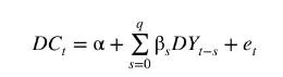
a. Use the observations in the data file cons_inc to estimate this model assuming \(q=4\). Use HAC standard errors. Comment on (i) the distribution of the lag weights and (ii) the significance of your estimates at a \(5 \%\) significance level.

b. Reestimate the equation, dropping the lags whose coefficients were not significant in part (a). Use HAC standard errors. Have there been any substantial changes in the estimates and standard errors of the coefficients of the retained lags?

c. Using an LM test with two lags, test for autocorrelation in the errors of the equation estimated in part (b). Is the use of HAC standard errors justified?

d. Assume that the errors follow the \(\mathrm{AR}(1)\) process \(e_{t}=ho e_{t-1}+v_{t}\) with the usual assumptions on \(v_{t}\). Transform the model estimated in part (b) into one that can be estimated using nonlinear least squares.

e. Use nonlinear least squares to estimate the model derived in part (d). Use HAC standard errors. Compare these estimates and their standard errors with those obtained in part (b).

f. Using the results from part (e), find an estimate for the total multiplier and its standard error. Compare these values with those obtained for the model in Example 9.16. (You will need to estimate the model in Example 9.16 to work out the standard error of its total multiplier.)

Data From Example 9.16:-

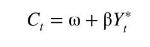
Suppose that consumption expenditure \(C\) is a linear function of "permanent" income \(Y^{*}\)

Permanent income is unobserved. We will assume that it consists of a trend term and a geometrically weighted average of observed current and past incomes, \(Y_{t}, Y_{t-1}, \ldots\)

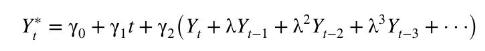
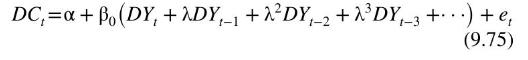
where \(t=0,1,2, \ldots\) is the trend term. In this model, consumers anticipate that their income will trend, presumably upwards, adjusted by a weighted average of their past incomes. For reasons that will become apparent in Chapter 12, it is convenient to consider a differenced version of the model where we relate the change in consumption \(D C_{t}=C_{t}-C_{t-1}\) to the change in actual income \(D Y_{t}=Y_{t}-Y_{t-1}\). This version of the model can be written as

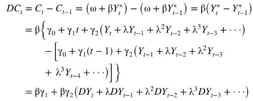
Setting \(\alpha=\beta \gamma_{1}\) and \(\beta_{0}=\beta \gamma_{2}\) and adding an error term, this equation, in more familiar notation, becomes

Its ARDL \((1,0)\) representation is

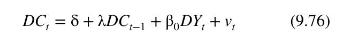
To estimate this model, we use quarterly data on Australian consumption expenditure and national disposable income from 1959Q3 to 2016Q3, stored in the data file cons_inc. Estimating (9.76) yields

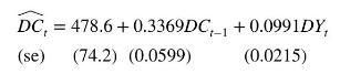
The delay multipliers from this model are \(0.0991,0.0334\), \(0.0112, \ldots\). The total multiplier is \(0.0991 /(1-0.3369)=\) 0.149. At first, these values may seem low for what could be interpreted as a marginal propensity to consume. However, because a trend term is included in the model, we are measuring departures from that trend. The LM test for serial correlation in the errors described in Section 9.4.2 was conducted for lags 1, 2, 3, and 4; in each case, a null hypothesis of no serial correlation was not rejected at a 5\% significance level. To see if this lack of serial correlation in the errors could be attributable to an \(\mathrm{AR}(1)\) model with parameter \(\lambda\) for the errors in (9.75), the steps for the test in the previous subsection were followed, yielding a test value of \(\chi^{2}=(T-1) \times R^{2}=227 \times 0.00025=0.057\). Given the \(5 \%\) significance level for a \(\chi_{(1)}^{2}\)-distribution is 3.84 , we fail to reject the null hypothesis that the errors in the IDL representation can be described by the process \(e_{t}=\lambda e_{t-1}+v_{t}\). Put another way, there is no evidence to suggest that the existence of an \(\mathrm{MA}(1)\) error of the form \(v_{t}=e_{t}-\lambda e_{t-1}\) is a source of inconsistency in the estimation of (9.76).

Transcribed Image Text:

DC, = a+B,DY+e, s=0