In Examples 9.14  and 9.15, we considered the Phillips curve

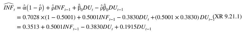
where inflationary expectations are assumed to be constant, \(I N F_{t}^{E}=\alpha\), and \(\beta_{0}=-\gamma\). In Example 9.15, we used data in the file phillips 5_aus to estimate this model assuming the errors follow an AR(1) model \(e_{t}=ho e_{t-1}+v_{t}\). Nonlinear least squares estimates of the model were \(\hat{\alpha}=0.7028, \hat{\beta}_{0}=-0.3830\), and \(\hat{ho}=0.5001\). The equation from these estimates can be written as the following ARDL representation (see equation (9.68))

Instead of assuming that this ARDL \((1,1)\) model is a consequence of an AR(1) error, another possible interpretation is that inflationary expectations depend on actual inflation in the previous quarter, \(I N F_{t}^{E}=\delta+\theta_{1} I N F_{t-1}\). If \(D U_{t-1}\) is retained because of a possible lagged effect, and we change notation so that it is line with what we are using for a general ARDL model, we have the equation

a. Find least squares estimates of the coefficients in (XR 9.21.2) and compare these values with those in (XR 9.21.1). Use HAC standard errors.

b. Reestimate (XR 9.21.2) after dropping \(D U_{t-1}\). Why is it reasonable to drop \(D U_{t-1}\) ?

c. Now, suppose that inflationary expectations depend on inflation in the previous quarter and inflation in the same quarter last year, \(I N F_{t}^{E}=\delta+\theta_{1} I N F_{t-1}+\theta_{4} I N F_{t-4}\). Estimate the model that corresponds to this assumption.

d. Is there empirical evidence to support the model in part (c)? In your answer, consider (i) the residual correlograms from the equations estimated in parts (b) and (c), and the significance of coefficients in the complete \(\operatorname{ARDL}(4,0)\) model that includes \(I N F_{t-2}\) and \(I N F_{t-3}\).

Data From Example 9.14:-

The Phillips curve has a long history in macroeconomics as a tool for describing the relationship between inflation and unemployment. \({ }^{11}\) Our starting point is the model

where \(I N F_{t}\) is the inflation rate in period \(t, I N F_{t}^{E}\) denotes inflationary expectations for period \(t, D U_{t}=U_{t}-U_{t-1}\) denotes the change in the unemployment rate from period \(t-1\) to period \(t\), and \(\gamma\) is an unknown positive parameter.

It is hypothesized that falling levels of unemployment \(\left(U_{t}-U_{t-1})\) reflect excess demand for labor that drives up wages which in turn drives up prices. Conversely, rising levels of unemployment \(\left(U_{t}-U_{t-1}>0\right)\) reflect an excess supply of labor that moderates wage and price increases. The expected inflation rate is included because workers will negotiate wage increases to cover increasing costs from expected inflation, and these wage increases will be transmitted into actual inflation. We assume that inflationary expectations are constant over time and set \(\alpha=I N F_{t}^{E}\). In addition, we set \(\beta_{0}=-\gamma\), and add an error term, in which case the Phillips curve can be written as the simple regression model

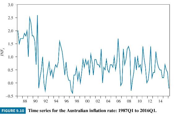
The data used for estimating (9.65) are quarterly Australian data from 1987, Quarter 1 to 2016, Quarter 1, a total of 117 observations, stored in the data file phillips5_aus. Inflation is calculated as the percentage change in the Consumer Price Index, with an adjustment in the third quarter of 2000 when Australia introduced a national sales tax. The adjusted

time series is graphed in Figure 9.10; the time series for the change in the unemployment rate was previously graphed in Figure 9.9. Tests for assessing whether these series are stationary are set as exercises in Chapter 12.
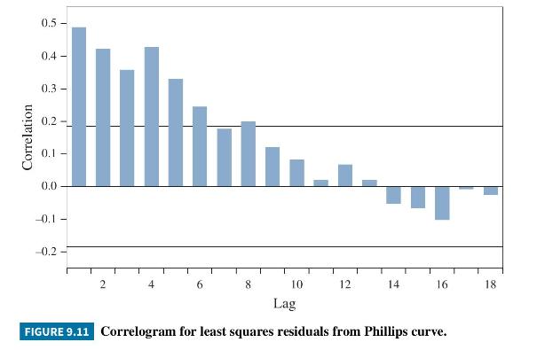
The correlogram of the residuals from least squares estimation of (9.65) is presented in Figure 9.11; approximate \(5 \%\) significance bounds for the autocorrelations are plotted at \(\pm 2 / \sqrt{117}= \pm 0.185\). There is evidence of moderate correlations at lags \(1-5\), and smaller ones at lags 6 and 8 . To examine the impact of the autocorrelated errors, in Table 9.9, we report the least squares estimates, and conventional (OLS), HCE and HAC standard errors, \(t\)-values, and

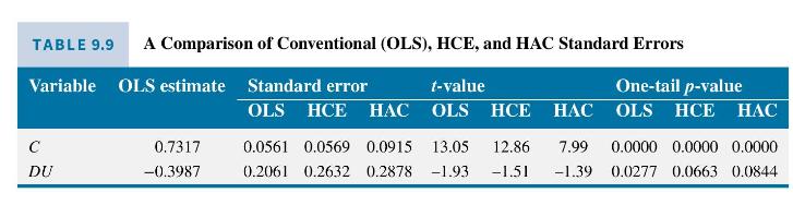
\(p\)-values. \({ }^{12}\) The HAC standard errors that allow for autocorrelation and heteroskedasticity are larger than the HCE standard errors that allow only for heteroskedacticity, and the HCE standard errors are larger than the conventional OLS ones that allow for neither heteroskedasticity nor autocorrelation. Thus, ignoring the autocorrelation and heteroskedasticity overstates the reliability of the least squares estimates. Overstating their reliability means that interval estimates will be narrower than they should be and we are more likely to reject a true null hypotheses. Using \(t_{(0.975,115)}=1.981,95 \%\) interval estimates for \(\beta_{0}\) are \((-0.8070,0.0096)\) with conventional standard errors and \((-0.9688,0.1714)\) with HAC standard errors. With conventional standard errors, a one-tail test and a 5\% significance level, we reject \(H_{0}: \beta_{2}=0\). With HCE or HAC standard errors, we do not reject \(H_{0}\).

Data From Equation 9.68:-

Data From Example 9.15:-

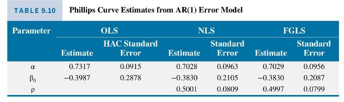
In this example, we obtain estimates of the Phillips curve introduced in Example 9.14 under the assumption that its errors can be modeled with an AR(1) process. The data file is phillips5_aus. We can, at the outset, conjecture that an AR(1) model might be inadequate. Returning to the correlogram of the least squares residuals in Figure 9.11, the first four sample autocorrelations are \(r_{1}=0.489\), \(r_{2}=0.358, r_{3}=0.422\), and \(r_{4}=0.428\). They do not decline exponentially, nor approximately so. Values that start from \(r_{1}=0.489\) and decline in line with the properties of an AR(1) model are \(r_{2}=0.489^{2}=0.239, r_{3}=0.489^{3}=0.117\), and \(r_{4}=0.489^{4}=0.057\). Nevertheless, we illustrate the AR(1) error model with this example and later, in Exercise 9.21, explore how we might improve it. Both the nonlinear least squares (NLS) and feasible generalized least squares (FGLS) estimates are reported in Table 9.10, along with the least squares (OLS) estimates and HAC standard errors reproduced from Table 9.9. The NLS and FGLS estimates and their standard errors are almost identical, and the estimates are also similar to those from OLS. The NLS and FGLS standard errors for estimates of \(\beta_{0}\) are smaller than the corresponding OLS HAC standard error, perhaps representing an efficiency gain from modeling the autocorrelation. However, one must be cautious with interpretations like this because standard errors are estimates of standard deviations,
themselves.

Transcribed Image Text:

INF, INFE-1(U,- U) + e = a + BDU, + e,