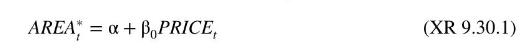
In this exercise, we consider a partial adjustment model as an alternative to the model used in Exercise 9.29 for modeling sugar cane area response in Bangladesh. The data are in the file bangla5. In the partial adjustment model long-run desired area, \(A R E A^{*}\) is a function of price,

In the short-run, fixed resource constraints prevent farmers from fully adjusting to the area desired at the prevailing price. Specifically,

where \(A R E A_{t}-A R E A_{t-1}\) is the actual adjustment from the previous year, \(A R E A_{t}^{*}-A R E A_{t-1}\) is the desired adjustment from the previous year, and \(0

a. Combine (XR 9.30.1) and (XR 9.30.2) to show that an estimable form of the model can be written as

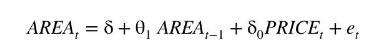
where \(\delta=\alpha \gamma, \theta_{1}=1-\gamma\), and \(\delta_{0}=\beta_{0} \gamma\).

b. Find least squares estimates of \(\delta, \theta_{1}\), and \(\delta_{0}\). Are they significantly different from zero at a \(5 \%\) significance level?

c. What are the first three autocorrelations of the residuals? Are they significantly different from zero at a \(5 \%\) significance level?

d. Find estimates and standard errors for \(\alpha, \beta_{0}\), and \(\gamma\). Are the estimates significantly different from zero at a \(5 \%\) significance level?

e. Find an estimate of \(A R E A_{73}^{*}\) and compare it with \(A R E A_{73}\).

f. Forecast \(A R E A_{74}, A R E A_{75}, \ldots, A R E A_{80}\) assuming that price in the next 7 years does not change from the last sample value \(\left(\right.\) PRICE \(_{74}=\) PRICE \(_{75}=\cdots=P R I C E_{80}=\) PRICE 73\()\). Comment on these forecasts and compare the forecast \(\widehat{A R E A}_{80}\) with \(A R E A_{80}^{*}\) estimated from (XR 9.30.1).

Data From Exercise 9.29:-

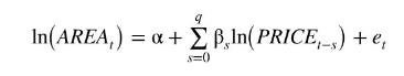
One way of modeling supply response for an agricultural crop is to specify a model in which area planted AREA depends on expected price, PRICE*. A log-log (constant elasticity) version of this model is \(\ln \left(\right.\) AREA \(\left._{t}\right)=\alpha+\gamma \ln \left(\right.\) PRICE \(\left._{t+1}^{*}\right)+e_{t}\) where PRICE \({ }_{t+1}^{*}\) is expected price in the next period when harvest takes place. When farmers expect price to be high, they plant more than when a low price is expected. Since they do not know the price at harvest time, we assume that they base their expectations on current and past prices, \(\ln \left(P R I C E_{t+1}^{*}\right)=\sum_{s=0}^{q} \gamma_{s} \ln \left(P R I C E_{t-s}\right)\), with more recent prices given a greater weight, \(\gamma_{0}>\gamma_{1}>\cdots>\gamma_{q}\). We use this model to explain the area of sugar cane planted in a region of the Southeast Asian country of Bangladesh. Information on the delay and interim elasticities is useful for government planning. It is important to know whether existing sugar processing mills are likely to be able to handle predicted output, whether there is likely to be excess milling capacity, and whether a pricing policy linking production, processing, and consumption is desirable. Data comprising 73 annual observations on area and price are given in the data file bangla5.

a. Let \(\beta_{s}=\gamma \gamma_{s}\). Show that the model can be written as the finite distributed lag model

b. Estimate the model in part (a) assuming \(q=3\). Use HAC standard errors. What are the estimated delay and interim elasticities? Comment on the results. What are the first four autocorrelations of the residuals? Are they significantly different from zero at a 5\% significance level?

c. You will have discovered that the lag weights obtained in part (a) do not satisfy a priori expectations. One way to try and overcome this problem is to insist that the weights lie on a straight line

If \(\alpha_{0}>0\) and \(\alpha_{1}

where \(z_{t 0}=\sum_{s=0}^{3} \ln \left(\right.\) PRICE \(\left._{t-s}\right)\) and \(z_{t 1}=\sum_{s=1}^{3} s \ln \left(P R I C E_{t-s}\right)\).

d. Create variables \(z_{t 0}\) and \(z_{t 1}\) and find least squares estimates of \(\alpha_{0}\) and \(\alpha_{1}\). Use HAC standard errors.

e. Use the estimates for \(\alpha_{0}\) and \(\alpha_{1}\) to find estimates for \(\beta_{s}=\alpha_{0}+\alpha_{1} s\) and comment on them. Has the original problem been cured? Do the weights now satisfy a priori expectations?

f. How do the delay and interim elasticities compare with those obtained earlier?

Transcribed Image Text:

AREA+BoPRICE, (XR 9.30.1)