Reconsider Example 11.2 on the supply and demand for fish at the Fulton Fish Market. The data are in the file fultonfish.

a. Add the variable MIXED, which indicates poor but not STORMY weather conditions, to the supply equation in equation (11.14). Estimate the new reduced-form equation for \(\ln (P R I C E)\), adding the variable MIXED to equation (11.16). Is it statistically significant at the \(5 \%\) level? Test the joint significance of STORMY and MIXED. Is the resulting \(F\)-value greater than 10 ?

b. Estimate the demand equation using STORMY and MIXED as IVs. Compare the coefficient estimates to those in Table 11.5.

c. Test the validity of the surplus instrument using the Sargan test, discussed in Section 10.3.4.

d. In the reduced-form equation in part (a), test the joint significance of the indicator variables \(M O N\), \(T U E, W E D\), and THU at the 5\% level. What do you conclude? Are we now able to estimate the supply equation by 2 SLS with confidence in our procedure?

Data From Example 11.2:-

The Fulton Fish Market has operated in New York City for over 150 years. The prices for fish are determined daily by the forces of supply and demand. Kathryn Graddy \({ }^{2}\) collected daily data on the price of whiting (a common type of fish), quantities sold, and weather conditions during the period December 2, 1991, to May 8, 1992. These data are in the file fultonfish. Fresh fish arrive at the market about midnight. The wholesalers, or dealers, sell to buyers for retail shops and restaurants. The first interesting feature of this example is to consider whether prices and quantities are simultaneously determined by supply and demand at all. \({ }^{3}\) We might consider this a market with a fixed, perfectly inelastic supply. At the start of the day, when the market is opened, the supply of fish available for the day is fixed. If supply is fixed, with a vertical supply curve, then price is demand-determined, with higher demand leading to higher prices but no increase in the quantity supplied. If this is true, then the feedback between prices and quantities is eliminated. Such models are said to be recursive and the demand equation can be estimated by OLS rather than the more complicated two-stage least squares procedure.
However whiting fish can be kept for several days before going bad, and dealers can decide to sell less, and add to their inventory, or buffer stock, if the price is judged too low, in hope for better prices the next day. Or, if the price is unusually high on a given day, then sellers can increase the day's catch with additional fish from their buffer stock. Thus despite the perishable nature of the product, and the daily resupply of fresh fish, daily price is simultaneously determined by supply and demand forces. The key point here is that "simultaneity" does not require that events occur at a simultaneous moment in time.

Let us specify the demand equation for this market as

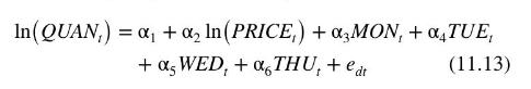
where \(Q U A N_{t}\) is the quantity sold, in pounds, and PRICE \({ }_{t}\) is the average daily price per pound. Note that we are using the subscript " \(t\) " to index observations for this relationship because of the time series nature of the data. The remaining variables are indicator variables for the days of the week, with Friday being omitted. The coefficient \(\alpha_{2}\) is the price elasticity of demand, which we expect to be negative. The daily indicator variables capture day-to-day shifts in demand. The supply equation is

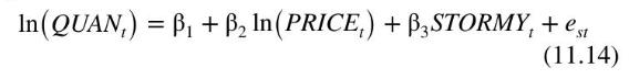
The coefficient \(\beta_{2}\) is the price elasticity of supply. The variable STORMY is an indicator variable indicating stormy weather during the previous three days. This variable is important in the supply equation because stormy weather makes fishing more difficult, reducing the supply of fish brought to market.

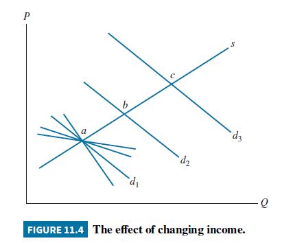
Prior to estimation, we must determine whether the supply and demand equation parameters are identified. The necessary condition for an equation to be identified is that in this system of \(M=2\) equations, it must be true that at least \(M-1=1\) variable must be omitted from each equation. In the demand equation the weather variable STORMY is omitted, and it does appear in the supply equation. In the supply equation, the four daily indicator variables that are included in the demand equation are omitted. Thus the demand equation shifts daily, while the supply remains fixed (since the supply equation does not contain the daily indicator variables), thus tracing out the supply curve, making it identified, as shown in Figure 11.4. Similarly, stormy conditions shift the supply curve relative to a fixed demand, tracing out the demand curve and making it identified.

The reduced-form equations specify each endogenous variable as a function of all exogenous variables

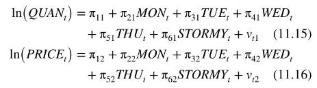
These reduced-form equations can be estimated by OLS because the right-hand side variables are all exogenous and uncorrelated with the reduced-form errors \(v_{t 1}\) and \(v_{t 2}\).

Using the Graddys' data (fultonfish), we estimate these reduced-form equations and report them in Tables 11.4a and \(11.4 \mathrm{~b}\). Estimation of the reduced-form equations is the first step of two-stage least squares estimation of the supply and demand equations. It is a requirement for successful two-stage least squares estimation that the estimated coefficients in the reduced form for the right-hand side endogenous variable be statistically significant. We have specified the structural equations (11.13) and (11.14) with \(\ln \left(Q U A N_{t}\right)\) as the left-hand side variable and \(\ln \left(P R I C E_{t}\right)\) as the right-hand side endogenous variable. Thus the key reduced-form equation is (11.16) for \(\ln \left(P R I C E_{t}\right)\). In this equation

- To identify the supply curve, the daily indicator variables must be jointly significant. This implies that at least one of their coefficients is statistically different from zero, meaning that there is at least one significant shift variable in the demand equation, which permits us to reliably estimate the supply equation.

- To identify the demand curve, the variable STORMY must be statistically significant, meaning that supply has a significant shift variable, so that we can reliably estimate the demand equation.
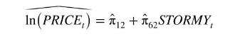
Why is this so? The identification discussion in Section 11.4 requires only the presence of shift variables, not their significance. The answer comes from a great deal of econometric research in the past decade, which shows that the two-stage least squares estimator performs very poorly if the shift variables are not strongly significant. \({ }^{4}\) Recall that to implement two-stage least squares we take the predicted value from the reduced-form regression and include it in the structural equations in place of the right-hand side endogenous variable, that is, we calculate 

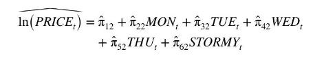
where \(\hat{\pi}_{k 2}\) are the least squares estimates of the reduced-form coefficients, and then replace \(\ln \left(P R I C E_{t}\right)\) with \(\widehat{\ln \left(P R I C E_{t}\right)}\). To illustrate our point, let us focus on the problem of estimating the supply equation (11.14) and take the extreme case that \ \hat{\pi}_{22}=\hat{\pi}_{32}=\hat{\pi}_{42}=\hat{\pi}_{52}=0\), meaning that the coefficients on the daily indicator variables are all identically zero. Then 

If we replace \(\ln \left(P R I C E_{t}\right)\) in the supply equation (11.14) with this predicted value, there will be exact collinearity between \(\widehat{\ln \left(\text { PRICE }_{t}\right)}\) and the variable STORMY \({ }_{t}\), which is already in the supply equation, and two-stage least squares will fail. If the coefficient estimates on the daily indicator variables are not exactly zero, but are jointly insignificant, it means there will be severe collinearity in the second stage, and although the two-stage least squares estimates of the supply equation can be computed, they will be unreliable. In Table 11.4b, showing the reduced-form estimates for (11.16), none of the daily indicator variables are statistically significant. Also, the joint \(F\)-test of significance of the daily indicator variables has \(p\)-value 0.65 , so that we cannot reject the null hypothesis that all these coefficients are zero. \({ }^{5}\) In this case the supply equation is not identified in practice, and we will not report estimates for it.

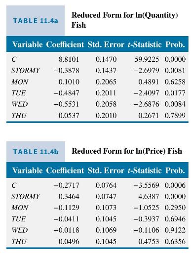
However, \(\operatorname{STORMY}_{t}\) is statistically significant in Table \(11.4 \mathrm{~b}\), meaning that the demand equation may be reliably estimated by two-stage least squares. An advantage of two-stage least squares estimation is that each equation can be treated and estimated separately, so the fact that the supply equation is not reliably estimable does not mean that we cannot proceed with estimation of the demand equation. The check of statistical significance of the sets of shift variables for the structural equations should be carried out each time a simultaneous equations model is formulated. 

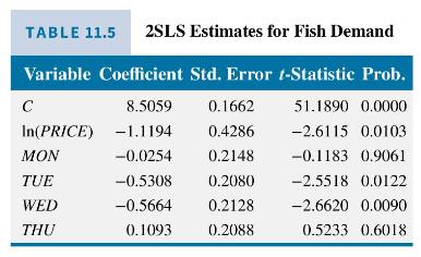
Applying two-stage least squares estimation to the demand equation we obtain the results as given in Table 11.5. The price elasticity of demand is estimated to be -1.12 , meaning that a \(1 \%\) increase in fish price leads to about a \(1.12 \%\) decrease in the quantity demanded; this estimate is statistically significant at the \(5 \%\) level. The indicator variable coefficients are negative and statistically significant for Tuesday and Wednesday, meaning that demand is lower on these days relative to Friday.

Data From Figure 11.4:-

 

Transcribed Image Text:

= In(QUAN,) + 2 In (PRICE,) +3 MON, + TUE, +s WED, + THU, + eat (11.13)