Several software companies report fixed effects estimates with an estimated intercept. As explained in Example 15.6, the

Question:

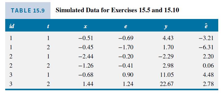
Several software companies report fixed effects estimates with an estimated intercept. As explained in Example 15.6, the value they report is the average of the coefficients of the indicator variables in the least squares dummy variable model, given in equation (15.17). Using the data in Table 15.9, the fitted dummy variable model is \(\hat{y}_{i t}=5.57 D_{1 i}+9.98 D_{2 i}+14.88 D_{3 i}+5.21 x_{i t}\).

a. Compute the average of the dummy variable coefficients, calling it \(C\).

b. The fitted fixed effects model, using the device from part (a), is \(\hat{y}_{i t}=C+5.21 x_{i t}\). Calculate \(\bar{y}_{i \bullet}-b_{2} \bar{x}_{2 i}\). for \(i d=1\) and \(i d=2\). For your convenience, to two decimals, \(\bar{y}_{1}=3.07, \bar{y}_{2 .}=0.34\) and \(\bar{x}_{1 .}=-0.48, \bar{x}_{2 .}=-1.85\). Round the calculated values to two decimals and compare them to the dummy variable coefficients.

c. Given the fitted model \(\hat{y}_{i t}=C+5.21 x_{i t}\), compute the residuals for \(i d=1\) and \(i d=2\).

d. What is the fitted within-model equation (15.17)?

e. Calculate the within-model residuals for \(i d=1\) and \(i d=2\).

f. Explain the relationship between the within model residuals in part

(e) and the residuals calculated in part (c), apart from any error caused by the two decimal rounding.

Data From Example 15.6:-

For the Chinese chemical firm data file chemical2, the indicator variable model in (15.21) becomes
\[\begin{aligned}\ln \left(\text { SALES }_{i t}\right)= & \beta_{11} D_{1 i}+\cdots+\beta_{1,200} D_{200, i}+\beta_{2} \ln \left(\text { CAPITAL }_{i t}\right) \\& +\beta_{3} \ln \left(\text { LABOR }_{i t}\right)+e_{i t}\end{aligned}\]
The fixed effects estimates of \(\beta_{2}\) and \(\beta_{3}\) will be identical to the within estimates in Example 15.4, and the standard errors will be the correct ones because in this indicator variable model the degrees of freedom are the correct \(N T-N-(K-1)=\) \(600-200-2=398\).
The \(N=200\) estimated indicator variable coefficients, \(b_{11}, b_{12}, \ldots, b_{1 N}\), may or may not be of specific interest. We include the indicator variables primarily to control for unobserved heterogeneity. If, however, we are interested in predicting the sales of a specific firm then the indicator variables become crucial. Given the estimates of \(\beta_{2}\) and \(\beta_{3}, b_{11}, b_{12}, \ldots\), \(b_{1 N}\) can be recovered using the fact that the fitted regression passes through the point of the means, just as it did in the simple regression model, that is, \(\bar{y}_{i .}=b_{1 i}+b_{2} \bar{x}_{2 i .}+b_{3} \bar{x}_{3 i}\), \(i=1, \ldots, N\). Reporting the estimates and their standard errors is inconvenient because \(N\) may be large. Software companies cope with this in different ways. Two popular econometric software programs, EViews and Stata, report a constant term \(C\) that is the average of the estimated coefficients on the cross-section indicator variables. For the Chinese chemical firm data, \(C=N^{-1} \sum_{i=1}^{N} b_{1 i}=7.5782\).
To test the null hypothesis \(H_{0}: \beta_{11}=\beta_{12}, \beta_{12}=\beta_{13}, \ldots\), \(\beta_{1, N-1}=\beta_{1 N}\), we use the sum of squared residuals from the fixed effects estimator, \(S S E_{U}=34.451469\), and from the pooled OLS regression

image text in transcribed

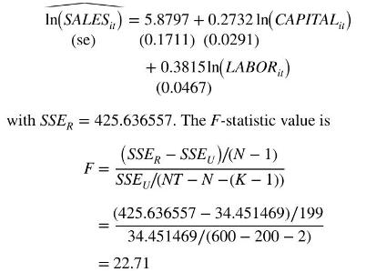
Using the \(\alpha=0.01\) level of significance, \(F_{(0.99,199,398)}=1.32\). We reject the null hypothesis and conclude that there are individual differences in the fixed effects constant terms for these \(N=200\) firms.

Data From Table 15.9:-

image text in transcribed